Whole-run plots

OutputPlots, from plasma_plots.output_accessors, works on a Struphy Output object rather than a single array, and gives you overview plots for a whole run. Struphy’s Output has it as out.plot, so out.plot() is a quick default (the scalar overview).

from struphy.post_processing.output import Output

out = Output("path/to/run")

out.plot.scalars(relative_to="initial", logy=True)
out.plot.equilibrium()
out.plot.equilibrium_3d(scalars="p0", cmap="viridis")

scalars(names=None, *, relative_to=None, logy=False) — plots every recorded scalar time series (e.g. field/kinetic energies) in one figure. Pass names to restrict to a subset, or relative_to to normalize each series against its initial value.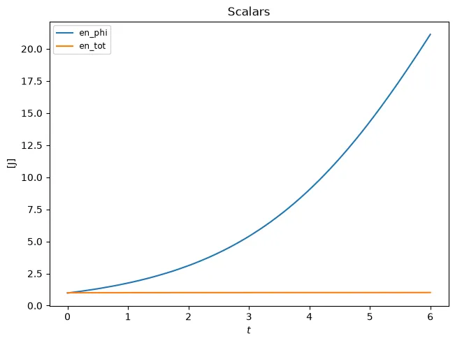

To write every scalar to disk at once, use plasma_plots.plotting.save_all_scalars(out.scalars, "plots/scalars"). It writes a CSV table, this overview, and one figure per scalar.
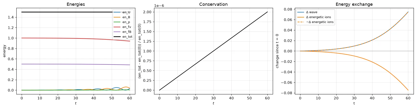
energies(parts=None, total="en_tot", groups=None) — the run’s energy budget: its energy scalars (en_*, or *_energy such as electric_energy in models that name them so), the relative drift of the total (which should stay flat), and with groups the energy exchanged between them. For a run with energetic ions driving a wave:
```
out.plot.energies(
    groups={
        "wave": ["en_U", "en_B", "en_p"],
        "energetic ions": ["en_fv", "en_fB"],
    }
)
```
Where energy only moves between the two groups, the wave’s gain and minus the ions’ change (dashed) overlap.
equilibrium(ax=None) — radial profiles of the run’s fluid equilibrium (out.equil, out.domain): pressure, and density/temperature if the equilibrium has a density profile too.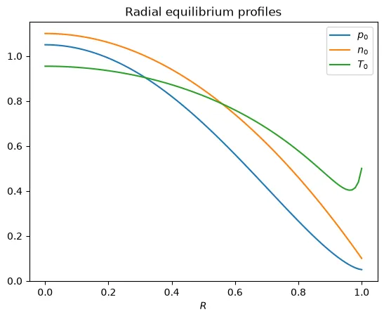
equilibrium_3d(scalars="p0", cmap="viridis") — interactive 3-D equilibrium view via PyVista. Requires pip install "plasma-plots[pyvista]".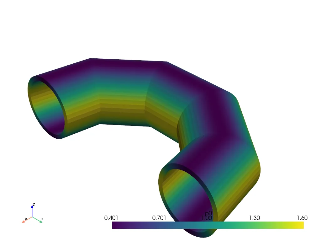
domain_3d(n1=8, n2=32, n3=32, surface=True) — a PyVista wireframe of the run’s mapping (out.domain), for checking its geometry. See 3-D views.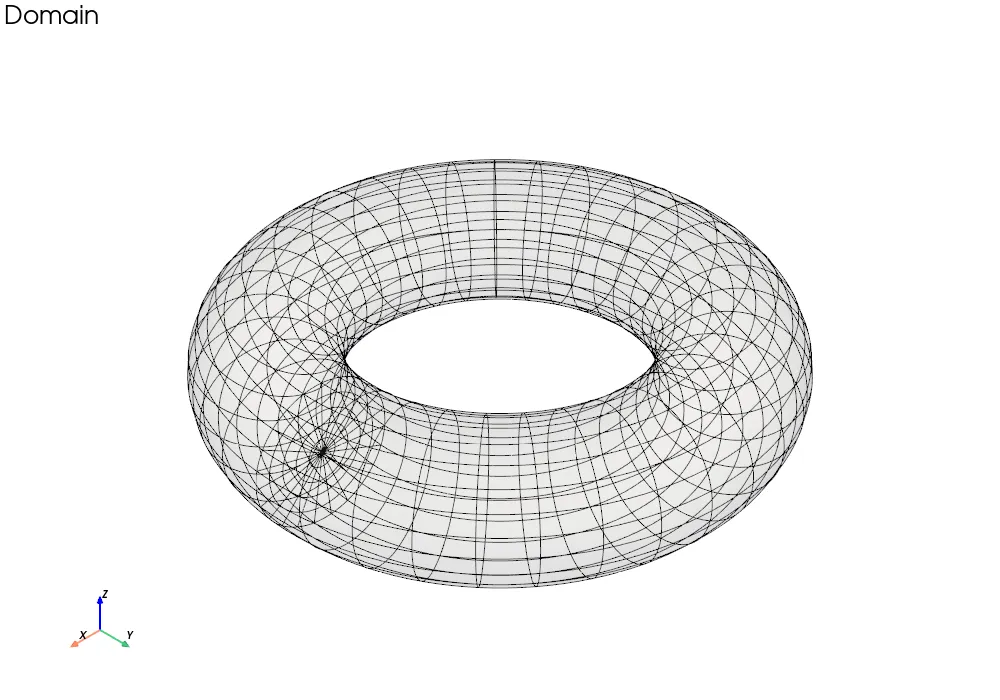

See the out.plot and out.analysis reference for full signatures.

Energies from fields

out.analysis.linear_mhd_energies() recomputes LinearMHD’s energy scalars (en_U, en_B, en_thermal, en_p, en_tot) from the saved fields. It uses the run’s mapping and equilibrium, at the Gauss points of every element. On real runs it matches the scalars Struphy saves during the simulation to machine precision. Its purpose is to measure the energy of fields that were never simulated, such as a filtered mode:

# Gauss points and weights per direction
etas, weights = out.analysis.quadrature_grid()
u = out.evaluate(
    "mhd/velocity",
    eta1=etas["eta1"],
    eta2=etas["eta2"],
    eta3=etas["eta3"],
    representation="2",
)
mode = u.plasma.analysis.filter_time(pad_bins=1).filtered
# energy in that mode
out.analysis.linear_mhd_energies(
    velocity=mode, b_field=None, pressure=None
).en_U

Fields must be in their FEEC space’s own representation: 2-form components for velocity and magnetic field, a 3-form for pressure. The default post-processing products use other representations ("norm", "0"). For other models, plasma_plots.analysis.field_energy and volume_integral compute the same kinds of integrals for any form. See the Diagnostics guide.