Dispersion spectrum
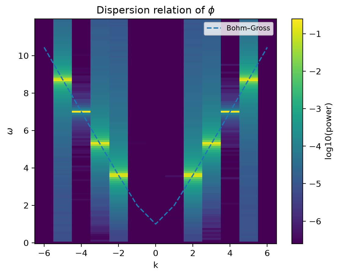
The dispersion relation from a time series: the – spectrum of a synthetic Langmuir wave field, with the theory curve drawn on it.
Four standing waves obeying plus noise are Fourier transformed in space and time; the spectrum has power only along the Bohm–Gross branch. The same call works on the output of a Vlasov or PIC run to see which branches a simulation actually carries.
Source code
Section titled “Source code”import matplotlib.pyplot as pltimport numpy as npimport xarray as xr
import plasma_plots # noqa: F401 (registers .plasma on DataArray)from plasma_plots.theory import kinetic
t = np.linspace(0.0, 60.0, 500)x = np.linspace(0.0, 2 * np.pi, 128, endpoint=False)X, T = np.meshgrid(x, t)
rng = np.random.default_rng(3)wave = 0.05 * rng.standard_normal(X.shape)for k in (2.0, 3.0, 4.0, 5.0): omega = kinetic.bohm_gross(k).real wave += np.cos(k * X - omega * T) + np.cos(k * X + omega * T)
phi = xr.DataArray( wave, dims=("t", "eta1"), coords={"t": t, "eta1": x}, name="phi", attrs={"label": r"$\phi$"},)phi.plasma.plot.dispersion( branches={"Bohm–Gross": kinetic.bohm_gross}, kmax=7, omega_max=12)plt.show()