3-D views
These views draw a field where it actually lives: on the physical X, Y,
Z points that every Struphy field product carries. On a mapped domain
(a torus, a cylinder, a stellarator) that is what makes them different from
the logical-coordinate field plots.
They need the optional PyVista extra:
pip install "plasma-plots[pyvista]"On this page, the 3-D figures have an Interactive 3-D view button that loads the
scene itself, exported with PyVista’s plotter.trame.export_html(...).
Each method returns a pyvista.Plotter without showing it. Call .show() in
a notebook or an interactive session, or .screenshot("view.png") in a batch
job (set pyvista.OFF_SCREEN = True first). To draw several views into one
scene, pass the plotter back in with plotter=. Dimensions other than eta1,
eta2, eta3 (and component for vectors) are selected by keyword, exactly as
for the 2-D plots, e.g. t=-1.
Isosurfaces
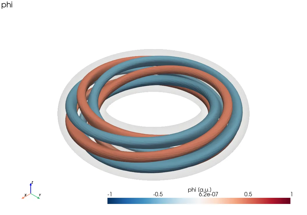
Section titled “Isosurfaces”phi.plasma.plot.isosurface(values=[-0.5, 0.5], cmap="RdBu_r", t=0)values is a number of evenly spaced levels or a list of explicit levels. The
domain boundary is drawn translucently for context (show_domain=False turns
it off).
Drag to rotate, scroll to zoom, shift-drag to pan.Open in a new tab
Cuts at fixed logical coordinates
Section titled “Cuts at fixed logical coordinates”slices_3d(cuts=...) draws surfaces of constant eta1, eta2 or eta3 where they
sit in physical space. On a torus, cuts in eta3 are poloidal cross-sections:
phi.plasma.plot.slices_3d( cuts={"eta3": [0, 0.25, 0.5, 0.75]}, cmap="RdBu_r", t=0)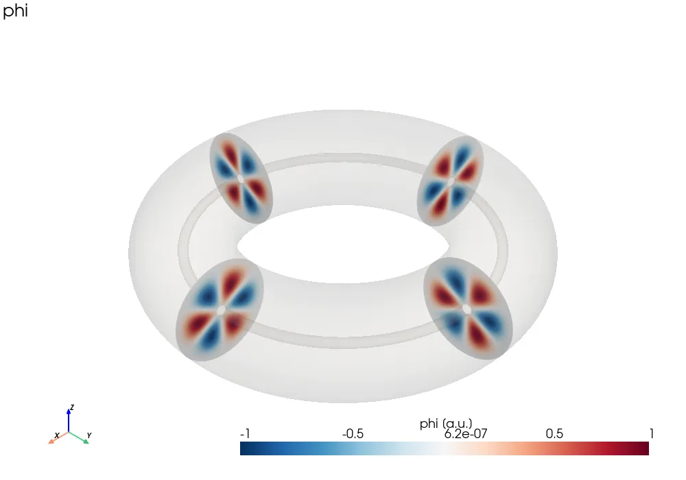
Drag to rotate, scroll to zoom, shift-drag to pan.Open in a new tab
A cut in eta1 shows the field on one flux surface, the usual way to see a
mode’s poloidal and toroidal structure:
phi.plasma.plot.slices_3d(cuts={"eta1": 0.5}, cmap="RdBu_r", t=0)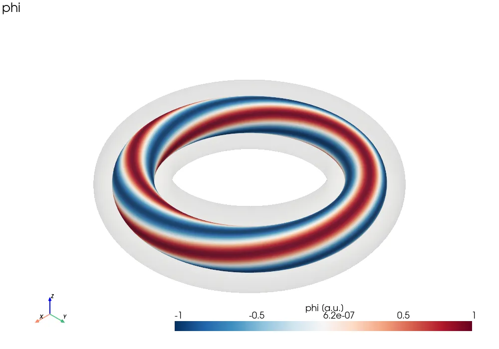
Drag to rotate, scroll to zoom, shift-drag to pan.Open in a new tab
Cut positions are logical coordinates (a float picks the nearest grid point),
or grid indices (integers, e.g. -1 for the last). Without cuts, the middle of
each direction is drawn. All cuts share one color scale.
Vector fields: field lines and arrows
Section titled “Vector fields: field lines and arrows”streamlines() traces field lines, e.g. of the magnetic field, from seeds in
a sphere around source_center:
b.plasma.plot.streamlines( n_points=60, source_center=(3.5, 0, 0), source_radius=0.35)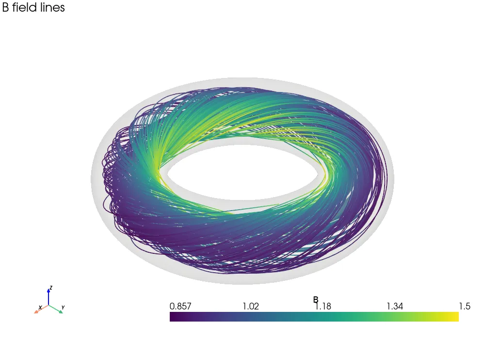
Drag to rotate, scroll to zoom, shift-drag to pan.Open in a new tab
glyphs() draws arrows colored by magnitude. stride thins the grid, and
selecting a single eta1 shows the field on one surface:
b.isel(eta1=[24]).plasma.plot.glyphs(stride=3, scale=0.5)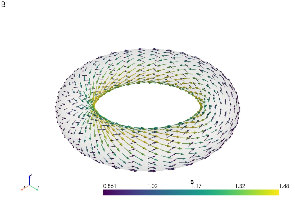
Drag to rotate, scroll to zoom, shift-drag to pan.Open in a new tab
Both expect Cartesian (x, y, z) components, as in the *_phy products of
out.pproc(physical=True). For contravariant logical components, e.g. from
out.evaluate(name, eta1=..., eta2=..., eta3=..., representation="v"), pass
components="contravariant". They are then pushed forward with the mapping’s
Jacobian, differentiated numerically from X, Y, Z
(plasma_plots.pyvista_plots.push_forward).
Orbits
Section titled “Orbits”orbits_3d() draws marker orbits as lines (or tubes, with tube_radius),
colored by time, by orbit class, or by
any saved quantity such as "v_par" or "weight". Samples where a marker has
left the domain are dropped. Pass any field as domain= to draw its boundary:
orbits.plasma.plot.orbits_3d(color_by="classification", domain=phi.isel(t=0))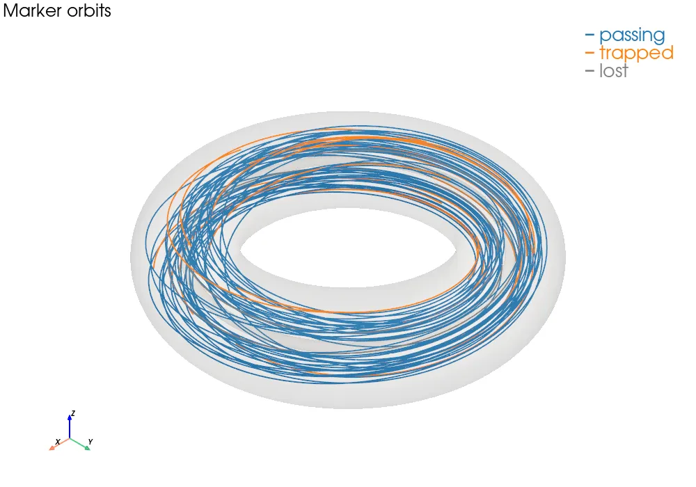
Drag to rotate, scroll to zoom, shift-drag to pan.Open in a new tab
The domain
Section titled “The domain”out.plot.domain_3d() draws a run’s mapping as a wireframe. The grid lines
cover the real boundary and, with cross_section=True (the default), the whole
eta3 = 0 face. Periodic seams and polar axes are left out. This is useful for
checking a geometry and its orientation:
out.plot.domain_3d(n1=6, n2=24, n3=36)# or, for any struphy domain object:from plasma_plots.pyvista_plots import pyvista_domain
pyvista_domain(domain, n1=6, n2=24, n3=36)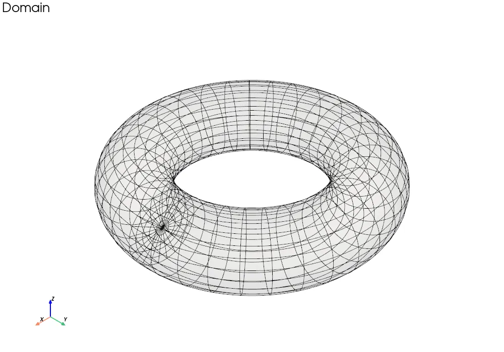
Drag to rotate, scroll to zoom, shift-drag to pan.Open in a new tab
2-D runs
Section titled “2-D runs”In a 2-D run one logical direction has a single grid point, or you have
selected it away (phi.isel(eta3=0)). The same methods then show the plane
itself, and the camera looks straight at it:
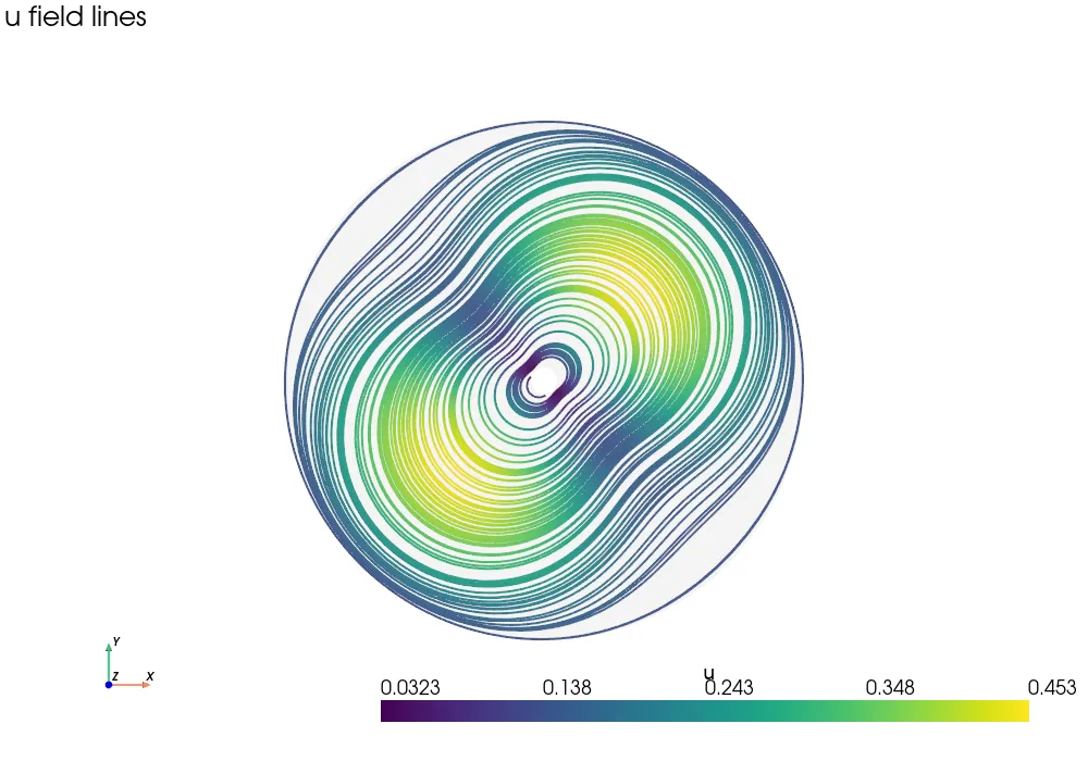
isosurface()draws the colored plane with contour lines.slices_3d()withoutcutsdraws the whole plane. Cuts through a plane are drawn as lines.streamlines()seeds on the plane and keeps the lines on it.glyphs()draws arrows in the plane.
phi.plasma.plot.isosurface(values=7, cmap="RdBu_r", t=0)u.plasma.plot.streamlines(n_points=80)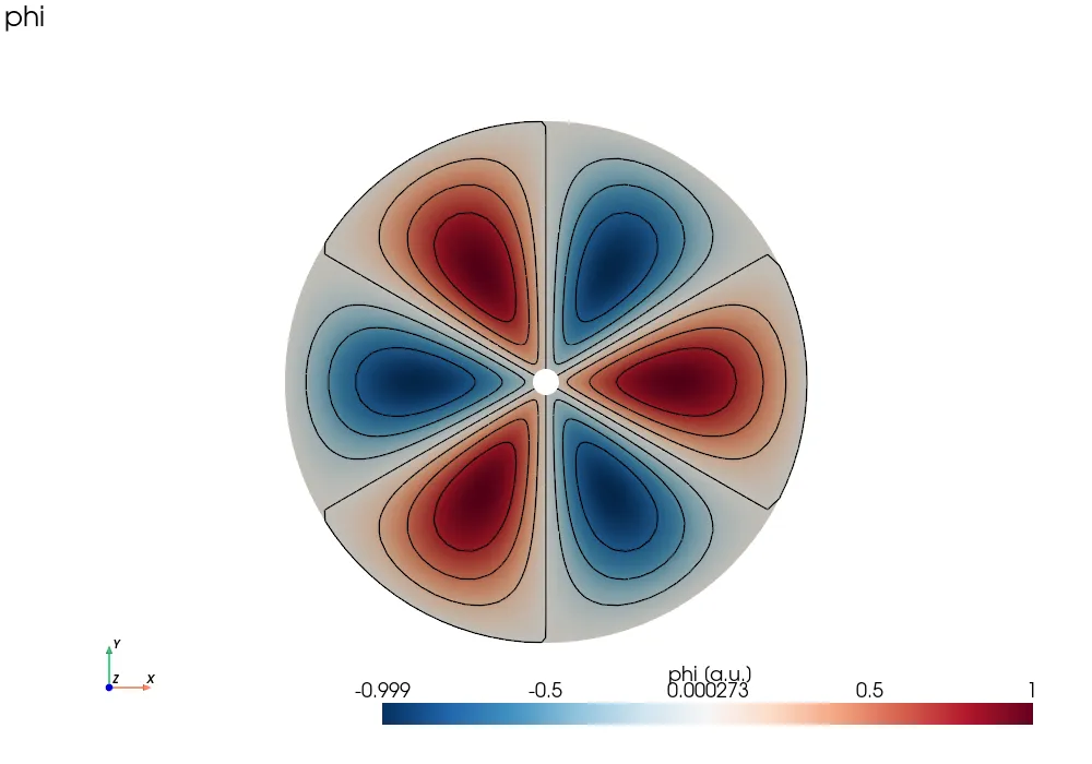
Movies
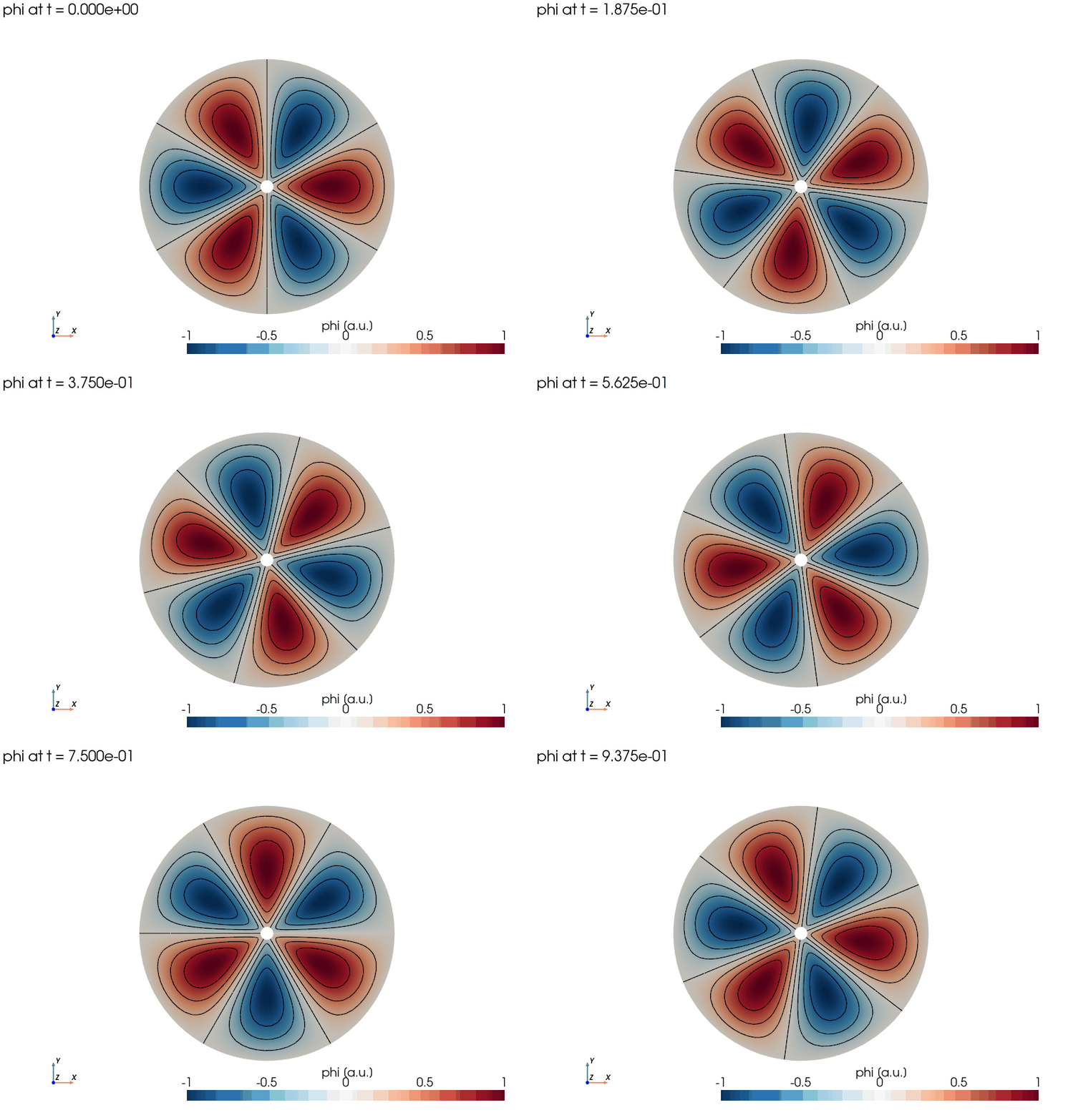
Section titled “Movies”movie() renders one 3-D view per time step into a GIF (needs imageio,
which comes with the pyvista extra) or a video such as .mp4 (needs
imageio-ffmpeg). Scalar views share one color scale over all frames, and the
camera stays fixed after the first frame:
phi.plasma.plot.movie( "mode.gif", kind="slices", cuts={"eta3": [0, 0.25, 0.5, 0.75]}, cmap="RdBu_r",)phi_2d.plasma.plot.movie( "mode_2d.gif", kind="isosurface", values=7, cmap="RdBu_r")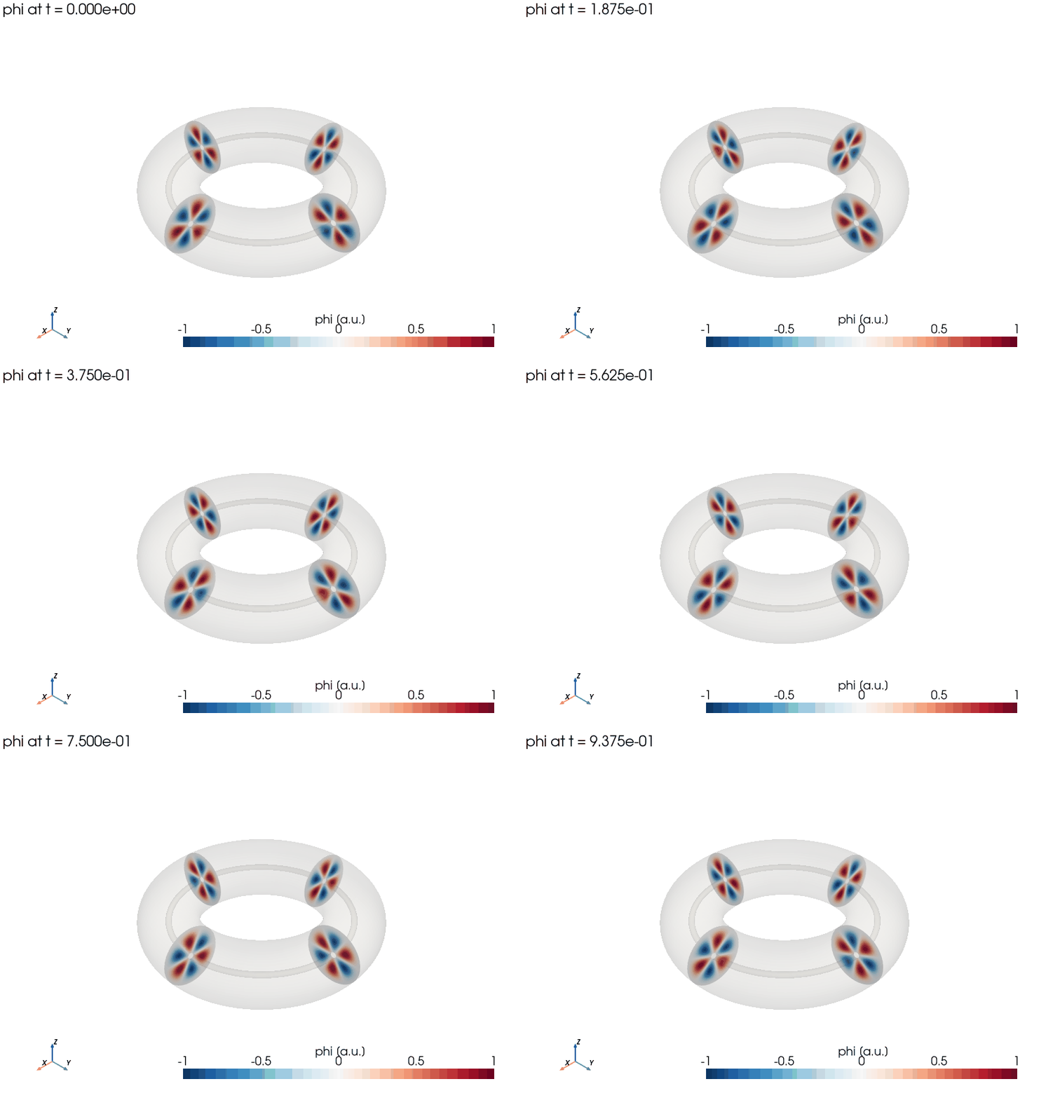
Your own PyVista pipeline
Section titled “Your own PyVista pipeline”field.plasma.data.grid(t=-1) returns the field as a
pyvista.StructuredGrid on its physical points. Vector fields also get their
magnitude as "|name|". You can hand the grid to any PyVista filter:
grid = phi.plasma.data.grid(t=-1)grid.contour([0.5]).plot(cmap="RdBu_r")For ParaView, field.plasma.data.to_vtk("frames") writes one .vts
structured grid per time and a .pvd collection that ParaView opens as a time
series. Any array works, e.g. a filtered mode from
filter_time(...).filtered.
To share a scene as a standalone web page, like the interactive views on this
page, export it with plotter.trame.export_html("scene.html"). This needs
pip install trame-pyvista, and with VTK 9.7 also trame-vtk 2.11.15 or
newer.