Command line

The plasma-plots command saves or displays figures of simulation output without writing any Python. It suits a first look at a run on a cluster, or a batch job that should leave figures behind. It opens:

• a Struphy run folder (it has run_metadata.json), as a Struphy Output;
• any file xarray can read: netCDF, zarr, … (GVEC evaluations are converted by themselves, as in GVEC equilibria).

pip install plasma-plots installs the command. For netCDF input, use pip install "plasma-plots[netcdf]"; see installation options. python -m plasma_plots runs the same thing.

plasma-plots info sim_1                                    # what is in it
plasma-plots plot sim_1 em_fields/phi slice t=-1 eta3=0 -o phi.png
plasma-plots movie sim_1 em_fields/phi eta3=0 -o phi.gif
plasma-plots quicklook sim_1 -o figures/                   # the standard figures

plasma-plots guide prints the package guide and plasma-plots api the API index. plasma-plots COMMAND --help lists the options of each command. Running plasma-plots without arguments also prints command help.

For a method’s signature, parameters and examples, no input file is needed:

plasma-plots help slice
plasma-plots help energies --kind run
plasma-plots help profile.gantt
plasma-plots help trajectories --kind dataset

You can also put --help after a selected method: plasma-plots plot run.nc phi slice --help. This does not open or process the run. Use --kind array, dataset, or run with the help command to choose a namespace when a method name exists in several places.

What is in it: info

plasma-plots info run.nc

File: run.nc

Variable  Dimensions                          Units  Description
--------  ----------------------------------  -----  ------------
phi       t: 81, eta1: 48, eta2: 64, eta3: 1  V      $\phi$
energy    t: 81                               J      field energy

Coordinate  Range
----------  ---------------
t           0 … 4 (81) s
eta1        0 … 1 (48)
eta2        0 … 0.9844 (64)
eta3        0 … 0 (1)

For a Struphy run, the table lists every product with its kind (scalar, field, distribution, density, orbits). These are the names that plot and movie accept.

One figure: plot

plot PATH PRODUCT METHOD key=value ... -o FILE calls PRODUCT.plasma.plot.METHOD(key=value, ...) and saves the result. The command has no plot options of its own, so every plot method works with the options documented for it (help(phi.plasma.plot.slice), or the reference):

plasma-plots plot run.nc phi slice t=-1 eta3=0 -o phi.png

Use --show to display a figure without saving it; -o is then optional:

plasma-plots plot run.nc phi slice t=-1 eta3=0 --show
plasma-plots movie run.nc phi eta3=0 --show
plasma-plots quicklook run.nc --show

Combine --show with -o to save and display. Matplotlib uses your configured interactive backend and waits until the window closes. Plotly figures open in your browser (backend=plotly). Quicklook displays each figure in turn; close its window to continue. File-writing methods such as frames and plot ... movie still require -o; use the movie command or an animation method to display an animation.

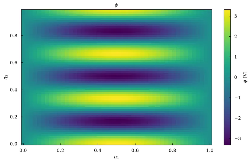
plasma-plots plot run.nc energy timeseries fit=[1,4] -o energy.png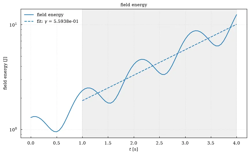

Name every dimension the plot doesn’t draw, as in Python: for a vector field that includes the component, e.g. plasma-plots plot sim_1 em_fields/e_field slice t=-1 eta3=0 component=0 -o e.png. A scalar time series is a product of its own: plasma-plots plot sim_1 electric_energy timeseries -o e.png.

plasma-plots plot PATH PRODUCT --list lists the methods a product has. Add --show to the listing to include interactive viewers and PyVista scenes. These methods require --show:

plasma-plots plot run.nc phi viewer eta3=0 --show
plasma-plots plot run.nc phi isosurface t=-1 --show
plasma-plots plot run.nc phi volume t=-1 --show -o volume.png

view opens its slider viewer. A viewer can also save its initial figure with -o; a PyVista scene can save a screenshot. PyVista requires the pyvista optional dependency. movie and frames write the file (or folder) given with -o themselves and do not accept --show; use the movie command or an animation method for display.

PRODUCT . stands for all of PATH: the run’s own plots (out.plot) for a Struphy folder, or the file’s Dataset (dataset.plasma.plot), e.g. for marker orbits:

plasma-plots plot sim_1 . energies -o energies.png
plasma-plots plot sim_1 . profile.gantt -o timeline.png

Option values

Values are read as Python values, with the selection rules of every plot (see Selecting data):

Typed	Value
t=-1, eta3=0	an integer: a position (the last, the first)
t=0.35	a decimal number: the nearest coordinate value
x=eta1	a string
logy=false, title=none	False, None
eta3=0,0.5	a list
fit=[1,4], cuts={"eta3":[0,0.5]}	JSON
other=@em_fields/B	another product of the same PATH

The format

The extension of -o picks the format: .png, .pdf, .svg (Matplotlib), or .html / .json. These last two draw with backend="plotly", as in Interactive plots, and need pip install "plasma-plots[plotly]". A Plotly figure saved as .png needs kaleido, and asks for it with backend=plotly. --dpi sets the resolution of images.

An animation: movie

movie PATH PRODUCT key=value ... -o FILE animates the product over t. It uses animation when two dimensions are left after the selection and line_animation when one is:

plasma-plots movie run.nc phi eta3=0 step=2 -o phi.gif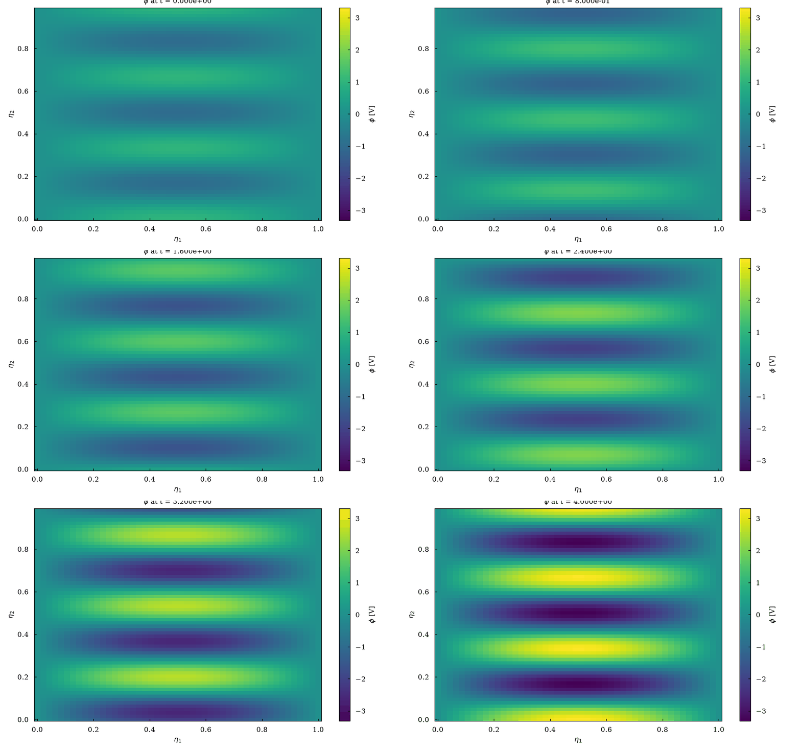

A .gif is written through Pillow and an .mp4 through ffmpeg (which must be installed). An .html file is an interactive Plotly animation with a slider. For a PyVista 3-D movie, call the method itself: plasma-plots plot PATH PRODUCT movie kind=slices -o movie.gif.

The standard figures: quicklook

plasma-plots quicklook sim_1 -o figures/
plasma-plots quicklook sim_1 -o figures/ --format png,html

To limit the work and choose a time, component or plane:

plasma-plots quicklook sim_1 --products em_fields/e_field em_fields/b_field --select t=-1 component=2 eta3=0 -o fields/
plasma-plots quicklook run.nc --products phi --select t=0.5 eta3=0 --show

--products omits run overview figures and draws only the named products. --select applies before choosing a slice, lineout or time series: integers select indices; decimals select the nearest coordinate. Each selection applies to products that have that dimension; a dimension absent from all selected products is an error. Without these options, the standard figures are:

• For a Struphy run: the energy budget (energies), the scalars, the equilibrium.
• For each field, distribution and density: a slice at t=-1 over its first two dimensions (logical ones first), at position 0 of the others, or a lineout when it has only one.
• For each orbits Dataset (or a file of markers): its trajectories.
• For each other time series of a file: a timeseries (a run’s scalars are in its scalar overview).

Profiling charts are generated explicitly, since a Gantt chart can be expensive for a long simulation:

plasma-plots plot sim_1 . profile.gantt -o timeline.png

A figure that fails is reported and skipped, and the others are still written. Files are named after the product and the plot, e.g. em_fields-phi-slice.png.

Struphy runs

The command automatically post-processes a run with the default options when needed and reuses existing processed output. No separate processing command is needed. To choose custom processing options, run struphy output pproc PATH first. Struphy’s own struphy output info and struphy output report describe the run’s data; plasma-plots draws it.

Errors exit with status 1; argument-parser errors exit with status 2. Messages suggest close method/product names, show dimensions for plotting errors, and point to method help. Basic argument mistakes are checked before opening or post-processing a run. --traceback shows where an error came from.

If --show cannot open a Matplotlib window, save with -o, choose backend=plotly --show for a browser figure, or configure an interactive Matplotlib backend with a working display. A noninteractive backend such as Agg now reports an error instead of silently returning without a window.

When to use Python instead

The command saves one plot per call, of one product. For figures of several panels (plasma_plots.figure), styling, derived arrays (phi - phi0, out.analysis), or data you pass as Python objects (reference= functions), write a script. The same calls work there: out.evaluate("em_fields/phi").plasma.plot.slice(t=-1, eta3=0).save("phi.png").