Charts and styles
These plots are not tied to a simulation grid. They take 1-D arrays over a
parameter or a category, Datasets of them, or plain dicts, and draw the charts
that otherwise end up as raw Matplotlib in notebooks: scans, budgets, profiles
with two axes, cross sections and system matrices. The functions behind them are
in plasma_plots.charts.
Parameter scans
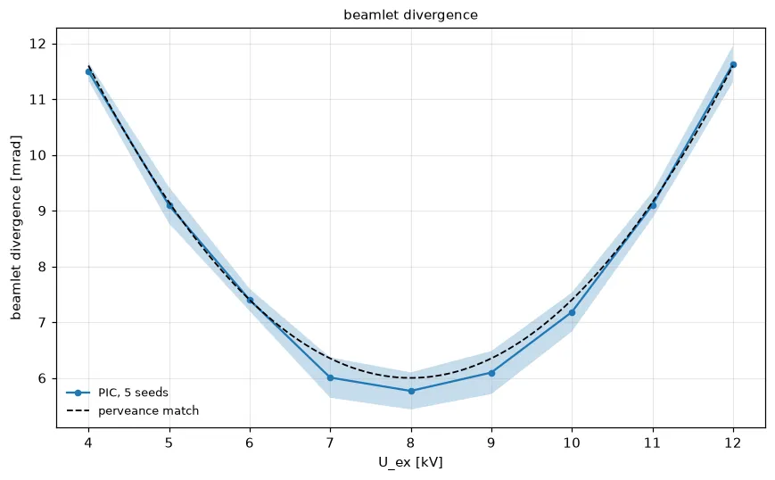
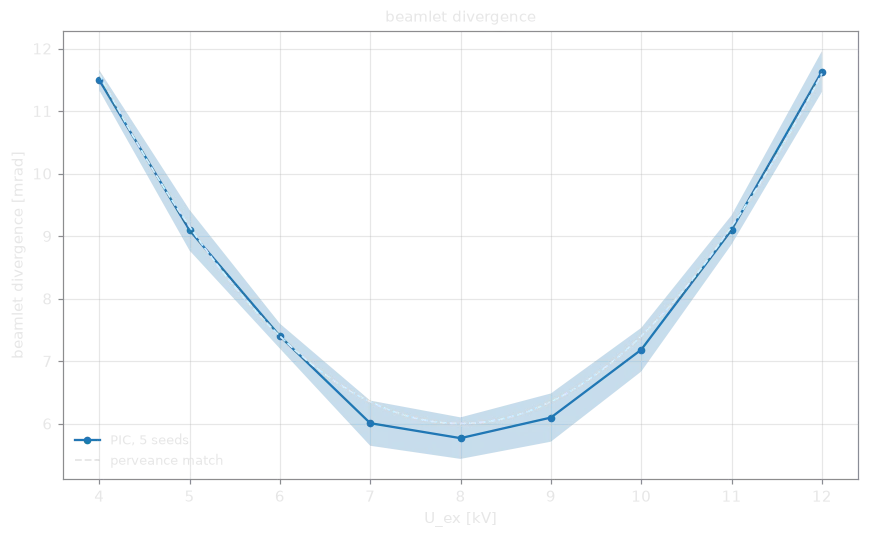
Section titled “Parameter scans”# divergence over (voltage, seed): the mean and spread of the seedsdivergence.plasma.plot.scan( samples="seed", band=True, label="PIC, 5 seeds", reference={"perveance match": lambda u: 6.0 + 0.35 * (u - 8.0) ** 2},)samples= names a dimension of repeated runs. The plot shows their mean, with
the standard deviation as error bars, or as a shaded band with band=True.
Without repeated runs, pass the errors yourself: error= takes a symmetric
error or a (lower, upper) pair. reference= adds expected curves, and
logx=, logy= and label= work as for the other plots, so several scans
share one axes with ax=.
divergence.plasma.data.scan(samples="seed") returns the values and errors as a
Dataset.
The same plot with Plotly
divergence.plasma.plot.scan(samples="seed", backend="plotly")
 Loading figure…
Breakdowns
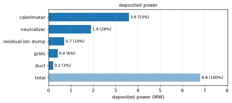
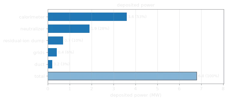
Section titled “Breakdowns”power.plasma.plot.breakdown( sort=True, total=True, scale=1e-6, xlabel="deposited power (MW)")Horizontal bars of the parts of a total, e.g. the power deposited on each
component of a beamline. The array runs over a category dimension, whose
coordinate names the bars. A Dataset of scalar variables works too
(deposited.plasma.plot.breakdown()), and so does a plain dict with
plasma_plots.charts.plot_breakdown({"duct": 0.2, "dump": 3.6}). Each bar is
annotated with its value and its share; sort=True puts the largest on top and
total=True adds the sum.
Two value axes and stacked panels
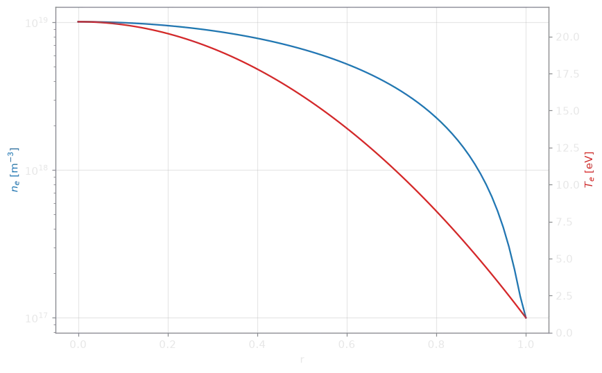
Section titled “Two value axes and stacked panels”n.plasma.plot.twin(T_e, logy=(True, False))Two profiles over the same coordinate, one value axis each, colored to match their lines.
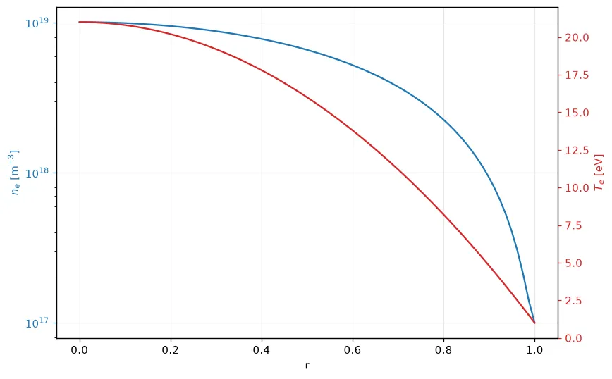
For more profiles, stack them in panels over a shared axis. A dict or list in a row draws several profiles together:
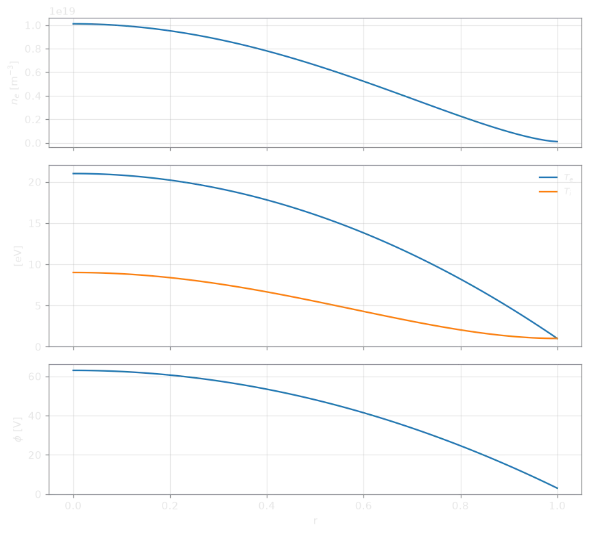
n.plasma.plot.stacked({"$T_e$": T_e, "$T_i$": T_i}, phi, t=-1)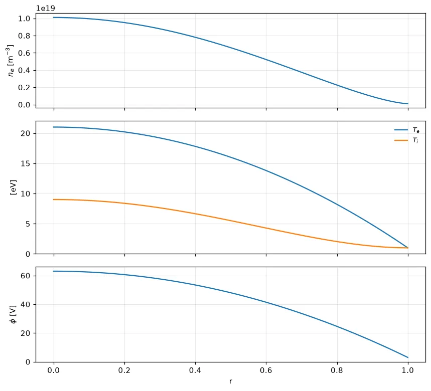
Every variable of a Dataset
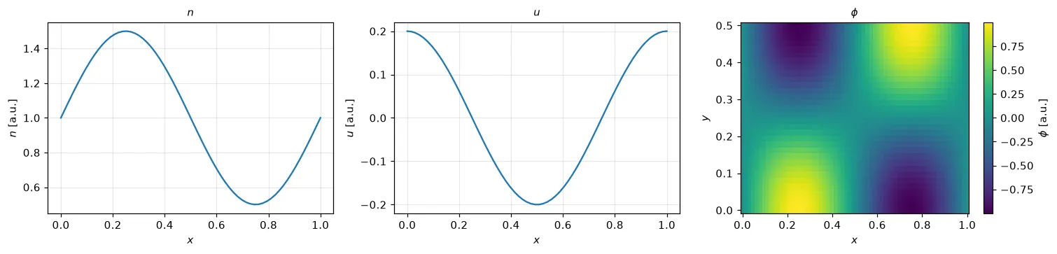
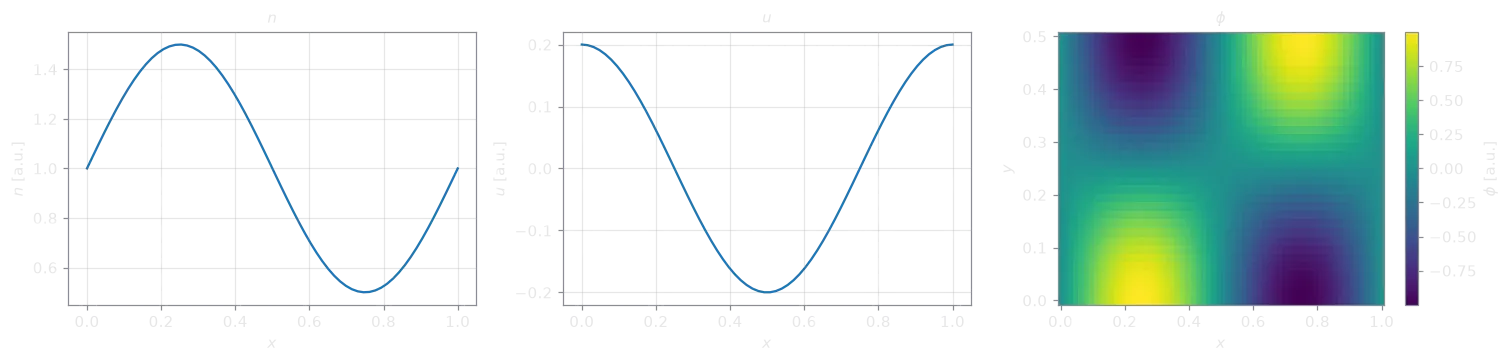
Section titled “Every variable of a Dataset”state.plasma.plot.variables(t=-1)One panel per variable, in a grid: a profile for a variable with one dimension
left after the selection, a slice for one with two. names= picks and orders
the variables, cols= sets the columns.
Cross sections
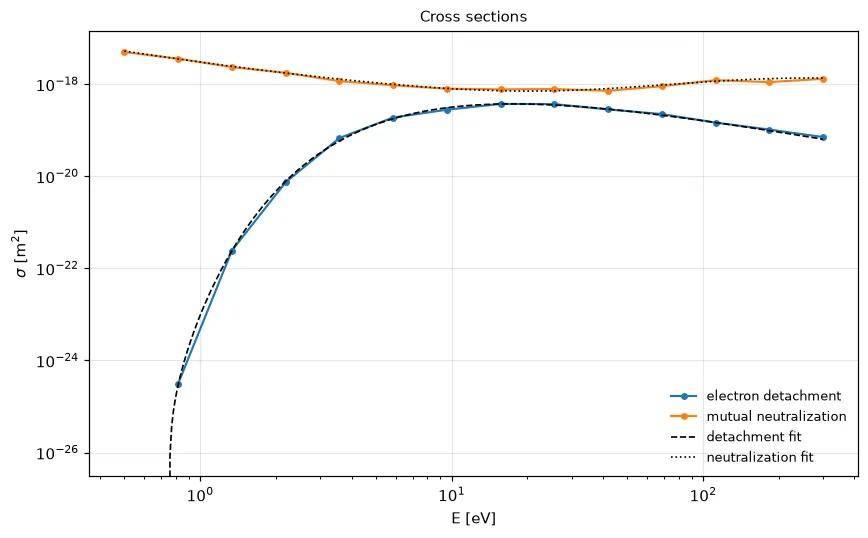
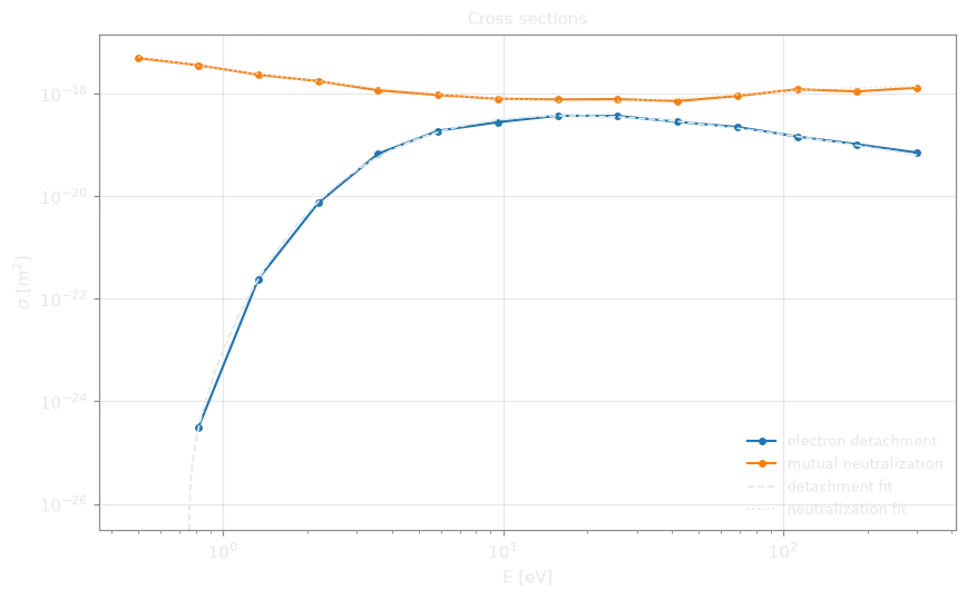
Section titled “Cross sections”catalogue.plasma.plot.cross_sections( reference={ "detachment fit": theory.negative_ions.electron_detachment_cross_section, "neutralization fit": theory.negative_ions.mutual_neutralization_cross_section, })Tabulated cross sections, or rate coefficients, over energy on log-log axes:
one line per Dataset variable, per entry of a process dimension, or per dict
entry. Non-positive values are left out on a log axis. reference= draws fits
or theory over the tabulated range.
Matrices
Section titled “Matrices”from plasma_plots.charts import plot_matrix
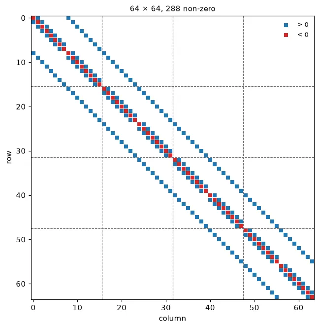
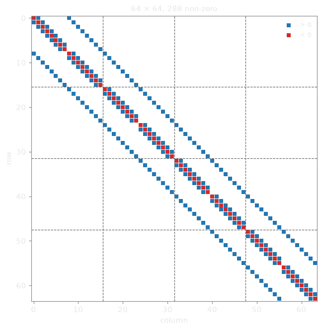
plot_matrix(A, rank_boundaries=[16, 32, 48])The non-zero pattern of a matrix, colored by sign, or with kind="values" its
entries on a symmetric color scale. It takes a dense array, a SciPy sparse
matrix, (rows, cols, values), or the dict picnic writes for a PETSc matrix
(row_indices, col_indices, values). rank_boundaries= marks where each
MPI rank’s rows begin. A 2-D DataArray has array.plasma.plot.matrix().
The Child–Langmuir law
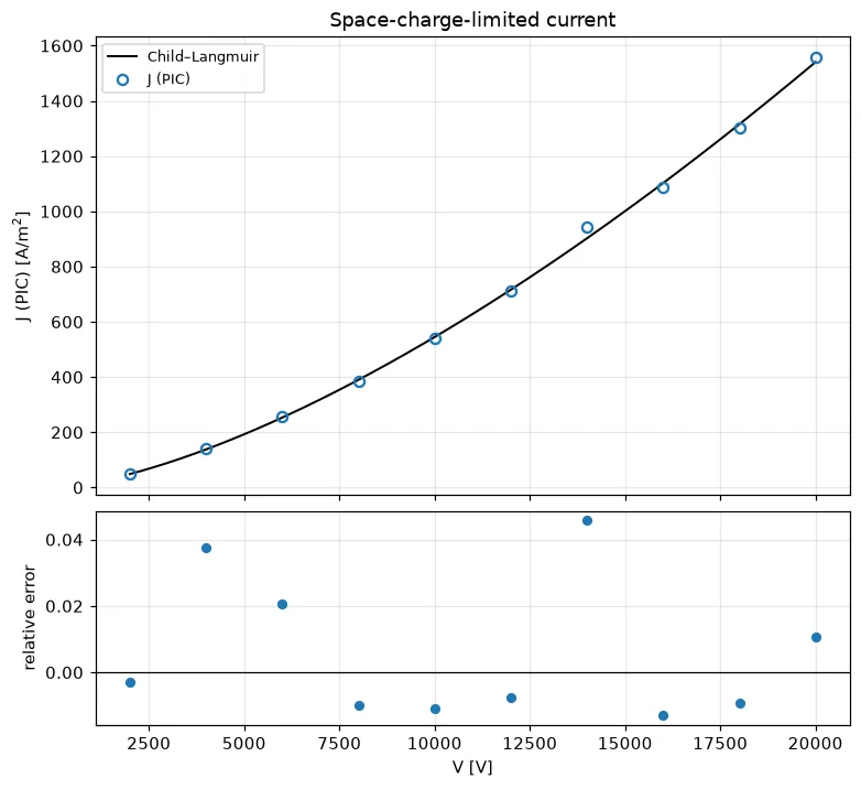
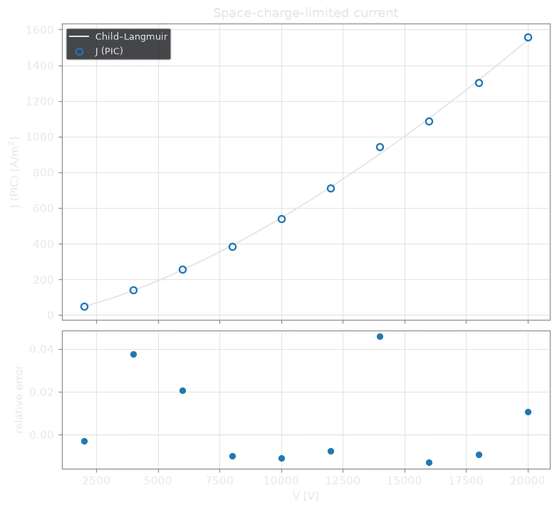
Section titled “The Child–Langmuir law”J.plasma.plot.child_langmuir(gap=0.01, mass=proton_mass)A current density over voltage, with gap=, or over the gap width, with
voltage=, against the space-charge limit of a planar diode, in SI units (see
child_langmuir). Further
arrays, e.g. from other codes, are compared in the same figure. The lower panel
shows the relative difference.
Styles
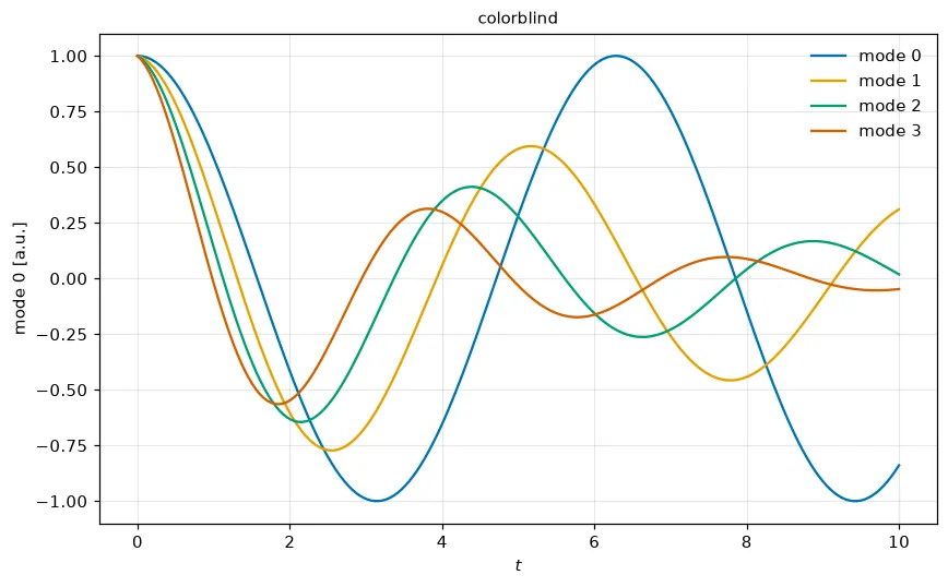
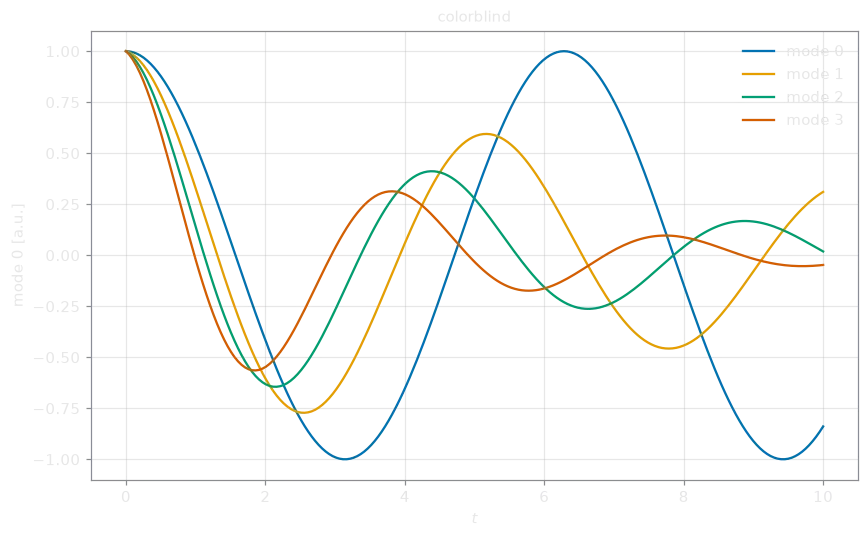
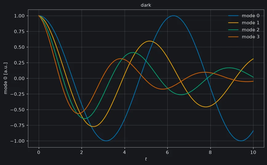
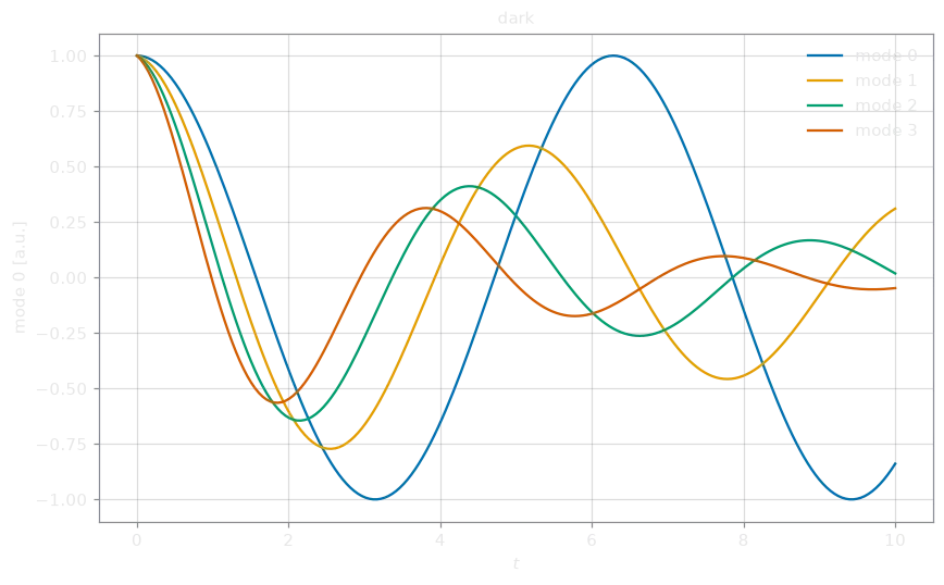
Section titled “Styles”plasma_plots.set_style("colorblind")with plasma_plots.style("dark"): energy.plasma.plot.timeseries().save("energy_dark.png")Every Matplotlib plot draws with the current style. set_style changes it for
every later plot, style for a with block, where it also applies to plain
Matplotlib figures. Keyword overrides change single rcParams, with
underscores for dots: set_style("paper", figure_dpi=300).
| Style | For |
|---|---|
"default" | the usual look |
"colorblind" | the default with the Okabe–Ito colors, which colour-blind readers tell apart |
"paper" | small figures with small text for a journal column, same colors |
"dark" | slides and dark pages |
"bare" | header pictures: no axes, labels or titles, transparent, the accent color first |
Front pages and embedding
Section titled “Front pages and embedding”For a docs front page, three exports strip a plot to its data:
from plasma_plots.hero import from_array
# an animated SVG header picture of a profile that changes over tfrom_array(phi.isel(y=0), tracer=True).save("docs/src/assets/hero.svg")# Plotly JSON or an HTML <div>, without axes, background or controlsresult = phi.plasma.plot.animation(x="x", y="y", eta3=0, backend="plotly")Path("hero.json").write_text(result.to_json(bare=True))html = energy.plasma.plot.timeseries().to_html()
to_json() and to_html() convert a Matplotlib result to Plotly first.
plotly_backend.bare does the
same stripping to any Plotly figure.