Diagnostics

These live on array.plasma.analysis, next to plotting on the same accessor, and return plain xarray objects or fit results rather than figures — plot them however you like. Full signatures are in the Analysis reference.

Growth and damping rates

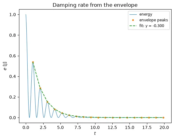
rate, amplitude = energy.plasma.analysis.growth_rate(window=(0.0, 5.0))
rate, amplitude = energy.plasma.analysis.damping_rate()

growth_rate fits an exponential directly; damping_rate fits the same exponential to the signal’s envelope first (analysis.envelope()), which is what you want for an oscillating-and-decaying signal such as the field energy in Landau damping — fitting the raw oscillation would give nonsense.

Damping rate fitted to the envelope of an oscillating, decaying signal

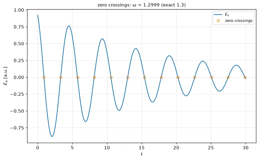
Oscillation frequency

oscillation_frequency() measures the frequency of one oscillation from its zero crossings, which damping or growth do not shift. Each crossing is interpolated to a fraction of a sample, and the period is the slope of a line through the crossing times, so a few periods give a frequency far finer than a spectrum’s bins:

fit = probe.plasma.analysis.oscillation_frequency(window=(0.0, 30.0))
fit.omega, fit.period, fit.times  # the crossings used
# from the maxima instead
probe.plasma.analysis.oscillation_frequency(method="peaks")

method="peaks" uses the maxima, for a signal that does not cross its mean. The peaks of an energy are half a period of the field apart, so they give twice its frequency. For several frequencies at once, use a spectrum.

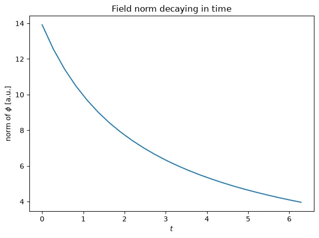
A damped oscillation with its zero crossings marked

Norm

field.plasma.analysis.norm(squared=False)

L2 norm over every dimension except t (or over dims explicitly), producing a (t,) series you can pass straight to .plasma.plot.lineout(x="t"):

Field norm decaying in time

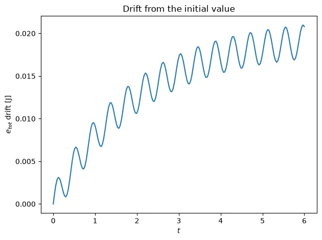
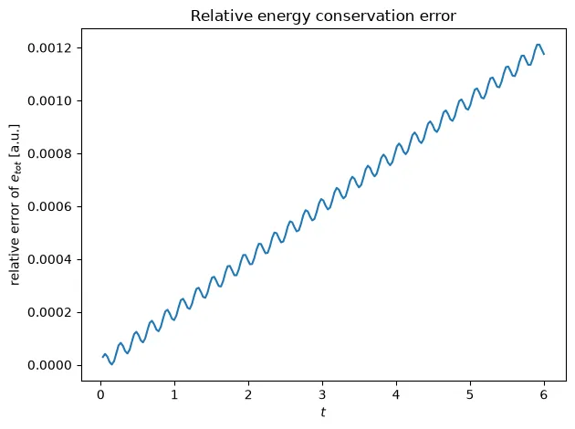
Drift and relative error

field.plasma.analysis.drift(ref=field.isel(t=0))
energy.plasma.analysis.relative_error(ref=exact_solution)

drift is the signed deviation from a reference (or the first sample); relative_error is the same, divided by the reference. Both return a (t,) series — handy for checking whether a conserved quantity actually stays conserved:

Drift of a scalar from its initial value

Relative energy-conservation error growing over a run

Errors against exact solutions

error() compares a field with an exact solution, given as an array or as a function of its coordinates. By default a function receives the physical X, Y, Z (or the logical dimensions if none are attached), then t. Name others with args=. The result is a function of the remaining dimensions, usually t:

exact = lambda x, t: heat_kernel(x, t)  # a 1-D profile over eta1 and t
T.plasma.analysis.error(exact, relative=True)  # relative RMS error over time
T.plasma.analysis.error(exact, norm="max")  # largest pointwise error
# the difference itself, for a slice plot
T.plasma.analysis.error(exact, norm="pointwise")

# ∫|u - u_exact|² dV
u.plasma.analysis.error(
    lambda x, y, z, t: np.sin(x - t), norm="l2", weighted=True
)

norm is "rms" (default), "max", "l1", "l2" or "pointwise", taken over dims (default: every dimension but t). Without weighting, the norms average over the grid points. On a mapped domain, such as a torus with a hollow core, this puts more weight on the inner points. weighted=True instead integrates over the physical volume with |√g| (taken from domain= or the X, Y, Z coordinates), which gives the proper L2 error. relative=True divides by the same norm of the exact solution.

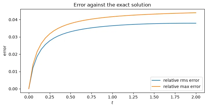
errors = [
    run.evaluate("T").plasma.analysis.error(exact).isel(t=-1) for run in runs
]
plot_convergence(resolutions, errors)

The relative error of the diffusing profiles in the field-plot guide, whose diffusion coefficient is 10 % too large:

Relative RMS and max errors against the exact solution, over time

plasma_plots.analysis.evaluate_on(field, function) gives the exact solution on the field’s points itself, e.g. for a reference in a slice plot.

Mode amplitudes by projection

project_mode() projects a field on one Fourier mode along a periodic direction: 2 ⟨f sin(2π n η / period)⟩ for kind="sin", the same with a cosine for kind="cos", and a complex amplitude (magnitude and phase) for kind="complex". It is the amplitude of a single known mode, as many examples compute by hand, without a full FFT:

# sine amplitude over t
amplitude = e1.plasma.analysis.project_mode(dim="eta1", number=1)
phase = np.angle(
    rho.plasma.analysis.project_mode(dim="eta2", number=3, kind="complex")
)

The grid has to cover one full period. For a binned distribution function, each bin averages the mode over its width, which lowers the amplitude by sinc(n h / period). bin_correction=True undoes this. For several modes at once, use the mode spectrum.

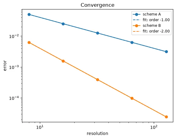
Convergence studies

errors = xr.DataArray(
    l2_errors, dims="n", coords={"n": [8, 16, 32, 64, 128]}, name="scheme A"
)
errors.plasma.plot.convergence(other_errors)  # fit the observed order of each
errors.plasma.plot.convergence(order=2)  # or draw a reference slope

plot.convergence draws 1-D errors over their resolution (or step size) log-log, one series per array, e.g. several schemes or norms. Give it an explicit order to draw a reference slope (e.g. 2 for an expected second-order scheme), or leave it to fit and report the observed order via plasma_plots.analysis.convergence_order. For plain arrays, plasma_plots.plotting.plot_convergence(resolutions, errors) does the same:

Two schemes’ error decaying with resolution, each with a fitted order

Distribution moments and spatial averaging

spatial_average() and velocity_moments() work on binned distribution products (f(t, eta1, v1) and similar) — see Particles & distributions for those, with figures.

Gradients on mapped domains

# Cartesian components (x, y, z), over time
E = -phi.plasma.analysis.gradient()
E.plasma.plot.vector(x="eta1", y="eta2", t=-1, eta3=0)

gradient() returns the Cartesian gradient J⁻ᵀ ∂f/∂η of a scalar field, with a component dimension in front of its own dimensions. The Jacobian comes from the X, Y, Z coordinates, or exactly from domain=out.domain. The logical derivatives are spectral around periodic angles, so on a torus the gradient is exact up to round-off. For a 2-D run it gives the gradient within the plane. The recipes use it for the E×B energy of drift waves and zonal flows.

Vector calculus

divergence() and curl() work like gradient(), on each Cartesian component (or on contravariant ones with components="contravariant", pushed forward first). They are spectral around periodic angles, so they are exact up to round-off on a torus:

B = out.evaluate("b_field_xyz")
div_B = B.plasma.analysis.divergence()  # should stay at round-off
J = B.plasma.analysis.curl()  # the current, in Cartesian components
vorticity = u.plasma.analysis.curl().sel(component=2)
div_B.plasma.analysis.norm().plasma.plot.timeseries()

flux_function() integrates an in-plane, divergence-free field (B_x = ∂A/∂y, B_y = −∂A/∂x) on a Cartesian slab or box to its flux function A (or the stream function of a flow), with zero mean. Its contour lines are the field lines, for example drawn over another field with contours_of:

A = B.plasma.analysis.flux_function()
J.sel(component=2).plasma.plot.slice(
    coords="physical", plane="XY", eta3=0, overlays={"contours_of": A}
)

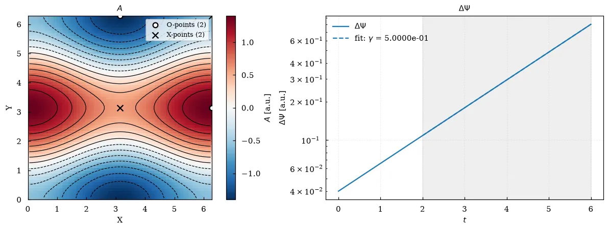
O-points, X-points and the reconnected flux

A = B.plasma.analysis.flux_function()
# (t, point): positions, values, kinds
points = A.plasma.analysis.critical_points()
A.plasma.plot.critical_points(t=-1, eta3=0)
flux = A.plasma.analysis.reconnected_flux(relative=False)
flux.plasma.plot.timeseries(fit=(10.0, 30.0))

The critical points of the flux function are where the gradient vanishes: critical_points finds every grid cell whose corners carry both signs of each gradient component, locates the zero of the gradient’s bilinear interpolant in it by Newton’s method (so the position is accurate to a fraction of a cell), and tells O-points (extrema, det H > 0) from X-points (saddles) by the Hessian. A periodic direction wraps when its coordinate has a period attribute or its physical coordinates close around; a plain periodic box without either is treated as bounded and loses the points on its edges. The plot marks the O-points as dots and the X-points as crosses on the flux contours.

reconnected_flux is the flux of the dominant island over time, |A(O) − A(X)| between an O-point and the X-point on its separatrix (the one nearest in flux), relative to the first time by default: for a tearing mode it grows as exp(γt), for the GEM challenge it is the usual reconnected-flux curve. o_point= and x_point= pin the pair to the points nearest given logical positions.

A tearing island: the flux contours with O-points and X-points, and the reconnected flux growing in time

Local components

For waves in a cylinder or torus, the Cartesian components are hard to read. cylindrical_components() rotates them to (R, phi, Z) about the Z axis. toroidal_components(R0=...) rotates them to (radial, poloidal, toroidal) about a circular axis at major radius R0 (and height Z0). Both need the X, Y, Z coordinates:

u = out.evaluate("velocity_xyz")
local = u.plasma.analysis.toroidal_components(R0=3.0)
local.sel(component="poloidal").plasma.plot.slice(
    coords="physical", plane="RZ", eta3=0, cmap="RdBu_r", symmetric=True
)

E = -phi.plasma.analysis.gradient()
E_R = E.plasma.analysis.cylindrical_components().sel(component="R")

polar_coordinates() attaches the radius r and angle theta about a center in the X-Y plane as coordinates, e.g. for profiles against the physical radius:

n_polar = n.plasma.analysis.polar_coordinates(center=(0.0, 0.0)).isel(
    t=-1, eta3=0
)
# average over rings of equal radius
radial_profile = n_polar.groupby_bins("r", 24).mean(...)

Volume integrals and field energies

from plasma_plots.analysis import field_energy, volume_integral

volume_integral(density)  # ∫ n dV, over time
field_energy(u_xyz)  # ½ ∫ |u|² dV of Cartesian components
# ½ uᵀ M2n u, as LinearMHD's en_U
field_energy(u_2form, form=2, weight=n0, domain=out.domain)

Both integrate over the logical grid with the volume element |√g|, as a function of every other dimension (e.g. t). form says what the array holds and sets the metric factor, as Struphy’s mass matrices do:

None or 0: a function or Cartesian components
1, 2, 3: p-form components
"v": contravariant components

The geometry comes from a Struphy domain (exact), or else from the Jacobian of the attached X, Y, Z coordinates. That Jacobian is differentiated spectrally around periodic directions, so a torus is exact up to round-off.

For quadrature, cell centers get the midpoint rule and other grids the trapezoidal rule. A spline field squared integrates exactly only with enough points per element, so for exact energies evaluate at the Gauss points of out.analysis.quadrature_grid() and pass its weights as quadrature=. See Energies from fields.

Dispersion relations

For time spectra, frequency filtering, mode numbers, eigenfunctions and growth rates from short records, see Spectral analysis.

field.plasma.plot.dispersion(
    dim="eta1", branches={"Bohm-Gross": lambda k: np.sqrt(1 + 3 * k**2)}
)

.plot.dispersion(...) is a plain space-time FFT of a (t, dim) field — independent of Struphy, so it works on any wave-like signal recorded over time along one spatial direction. dim defaults to the sole dimension other than t; select every other dimension away first (e.g. component, eta2, eta3). branches optionally overlays named theoretical curves — a mapping of label to a callable omega(k), or an explicit (k, omega) pair — to compare the measured ridge against theory:

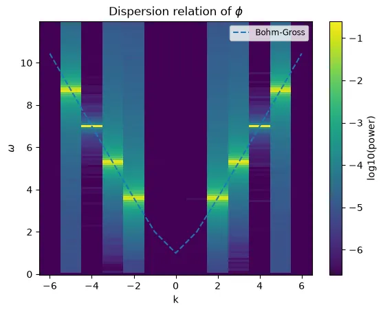
A dispersion relation recovered from a space-time FFT, with the Bohm-Gross branch overlaid

A dispersion relation’s power spans many orders of magnitude (the ridge against an otherwise near-empty plane), so .plot.dispersion(...) defaults its color limits to the top dynamic_range=6 decades below the peak rather than the full range down to numerical noise — pass vmin/vmax yourself if the ridge still looks washed out, or kmax/omega_max to zoom into it.

.plasma.analysis.dispersion(...) (or the matching .plasma.data.dispersion(...)) returns just the (omega, k) power spectrum, an xarray.DataArray, without plotting it — see plasma_plots.analysis.power_spectrum for the exact definition (a detrended 2-D FFT).

The same plot with Plotly

The same call with backend="plotly": an interactive figure with the same data, fits and labels (see Interactive plots with Plotly).

field.plasma.plot.dispersion(
    dim="eta1",
    branches={"Bohm-Gross": lambda k: np.sqrt(1 + 3 * k**2)},
    backend="plotly",
)

Loading interactive chart…

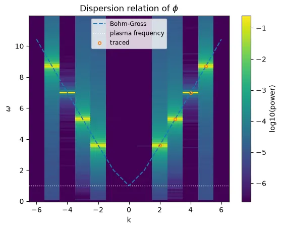
Tracing a branch

trace_branch() follows a branch through the (omega, k) spectrum. It needs a theory guess omega(k), and for each k it takes the strongest frequency within a relative window of that guess. Waves moving in either direction count, because the power at −k is added. The result is a Dataset over k with the measured omega, omega_theory and their relative_error:

spectrum = phi.plasma.analysis.dispersion()
traced = spectrum.plasma.analysis.trace_branch(
    bohm_gross, window=0.2, k_range=(1.5, 5.5)
).dropna("k")
phi.plasma.plot.dispersion(
    branches={"Bohm-Gross": bohm_gross},
    frequencies={"plasma frequency": 1.0},
    points={"traced": traced},
)

frequencies draws horizontal lines at fixed frequencies (e.g. a cutoff or the plasma frequency). points marks measured (k, omega) values, as a Dataset or DataArray from trace_branch or as a pair of arrays.

The Bohm-Gross branch, traced, with the plasma frequency

To compare the traced frequencies with the theory, and see their errors, use against_theory: traced.omega.plasma.plot.against_theory(bohm_gross).

Fitting straight branches

Without a theory to guide the search, fit_branches() fits omega = v k to each of several straight ridges, e.g. light waves or sound waves excited at once. .plot.dispersion takes the spectrum itself as well as the field, draws the fits dotted with fits=, and kmin=0 keeps the positive quadrant, where the fits were made:

spectrum = e_x.plasma.analysis.dispersion(dim="z")
fits = spectrum.plasma.analysis.fit_branches(n_branches=1)
fits[0].velocity  # ≈ 1, the speed of light
spectrum.plasma.plot.dispersion(
    kmin=0,
    branches={"light, ω = k": lambda k: k},
    fits=fits,
    dynamic_range=12,
    omega_max=25,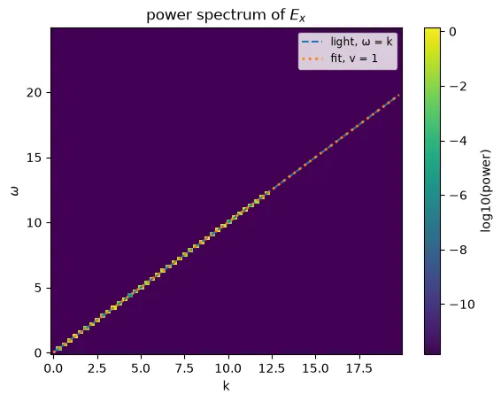
)

Broadband light waves, with the theoretical and the fitted branch

The same plot with Plotly

The same call with backend="plotly": an interactive figure with the same data, fits and labels (see Interactive plots with Plotly).

spectrum.plasma.plot.dispersion(
    kmin=0,
    branches={"light, ω = k": lambda k: k},
    fits=fits,
    dynamic_range=12,
    omega_max=25,
    backend="plotly",
)

Loading interactive chart…