MHD slab waves
An example of plasma_plots on a real struphy run, rather than the small synthetic data
used elsewhere in these docs — adapted from struphy’s own
MHD slab waves gallery example.
Selected pieces of the script appear below; the full file is folded at the end. For many
more worked examples, see the Struphy examples gallery.
The physics
Section titled “The physics”struphy.models.LinearMHD, in a uniform, obliquely magnetized plasma
(struphy.fields_background.equils.HomogenSlab, background field B0 = (0, 1, 1)).
Broadband noise in the velocity excites every MHD wave branch along z at once: the shear
Alfvén wave, and the slow and fast magnetosonic waves. Their exact ideal-MHD speeds follow
from the background alone; comparing them against the speeds actually measured from the
run’s own output is the point of the two figures below.
# The background: B0 = (0, 1, 1), density 0.7, plasma beta 3 (thermal over
# magnetic pressure).
B0x, B0y, B0z = 0.0, 1.0, 1.0
n0, beta, gamma = 0.7, 3.0, 5.0 / 3.0
B_squared = B0x**2 + B0y**2 + B0z**2
p0 = beta * B_squared / 2.0

# The exact ideal-MHD wave speeds along z, to compare the measured ones
# against.
alfven_speed = np.sqrt(B_squared / n0)
sound_speed = np.sqrt(gamma * p0 / n0)
cs2, va2 = sound_speed**2, alfven_speed**2
delta = 4 * B0z**2 * cs2 * va2 / ((cs2 + va2) ** 2 * B_squared)
exact_speeds = {
    "shear Alfven": alfven_speed * B0z / np.sqrt(B_squared),
    "slow magnetosonic": np.sqrt(0.5 * (cs2 + va2) * (1 - np.sqrt(1 - delta))),
    "fast magnetosonic": np.sqrt(0.5 * (cs2 + va2) * (1 + np.sqrt(1 - delta))),
}
Reproducing it
Section titled “Reproducing it”This needs the full compiled struphy runtime (pip install "struphy>=3.4.0", followed by
struphy compile -y) — see
CONTRIBUTING.md.
The run itself takes under a minute. Once it’s been run once, pass --pproc-only to redo
just the measurement and plotting below against the existing output, without rerunning the
simulation.
def run_simulation() -> Output:

    model = LinearMHD()
    model.propagators.shear_alf.options = model.propagators.shear_alf.Options(
        algo="implicit"
    )
    for component in range(3):
        model.mhd.velocity.add_perturbation(
            perturbations.Noise(amp=0.1, comp=component, seed=123)
        )
    equil = equils.HomogenSlab(B0x=B0x, B0y=B0y, B0z=B0z, beta=beta, n0=n0)

    sim = Simulation(
        model=model,
        env=EnvironmentOptions(sim_folder="mhd_slab_waves"),
        time_opts=Time(dt=0.15, Tend=180.0),
        domain=domains.Cuboid(r3=60.0),
        grid=grids.TensorProductGrid(num_elements=(1, 1, 64)),
        derham_opts=DerhamOptions(degree=(1, 1, 3)),
        equil=equil,
    )
    out = sim.run()
    return out
Measuring the branches
Section titled “Measuring the branches”Both fields are evaluated at a single point in the cross-section, physical z as the
remaining spatial coordinate, and turned into a space-time power spectrum with
.plasma.analysis.dispersion(). .plasma.analysis.fit_branches(...) then fits a straight
omega = v * k ridge to each branch — restricted to k between 0.2 and 2.0, since that’s
where these branches are actually linear and cleanly separated: past k ~ 2-2.5 the ridges
visibly bend, a real numerical-dispersion effect of this degree-3 spline discretization, not
a resolution or plotting artifact. That window has to stay a fixed k range rather than a
fraction of the grid’s own Nyquist k, since a finer grid only pushes the Nyquist limit
out — it doesn’t move where the physics stops being linear. The pressure fit also needs an
unusually low noise_level: the fast branch’s power there is only a few percent of the slow
branch’s peak power, so a more typical threshold would miss it entirely.
def pproc(out: Output):
    # Both fields are evaluated at a single (eta1, eta2) point, physical z as
    # the remaining spatial coordinate (logical eta3 swapped for physical Z, so
    # k comes out in physical units, matching the exact speeds above).
    velocity = out.evaluate("mhd/velocity", component=0).isel(eta1=0, eta2=0)
    velocity = velocity.assign_coords(eta3=("eta3", velocity["Z"].values))
    pressure = out.evaluate("mhd/pressure").isel(eta1=0, eta2=0)
    pressure = pressure.assign_coords(eta3=("eta3", pressure["Z"].values))

    velocity_spectrum = velocity.plasma.analysis.dispersion(dim="eta3")
    pressure_spectrum = pressure.plasma.analysis.dispersion(dim="eta3")

    fit_k_range = (0.2, 2.0)
    (alfven_branch,) = velocity_spectrum.plasma.analysis.fit_branches(
        n_branches=1, k_range=fit_k_range, noise_level=0.5
    )
    # The fast branch's power is only a few percent of the slow branch's peak
    # power in this window, so noise_level has to be low enough to still count
    # it as a genuine peak.
    slow_branch, fast_branch = pressure_spectrum.plasma.analysis.fit_branches(
        n_branches=2, k_range=fit_k_range, noise_level=0.02
    )
    measured_alfven, measured_slow, measured_fast = (
        alfven_branch.velocity,
        slow_branch.velocity,
        fast_branch.velocity,
    )
    measured_speeds = {
        "shear Alfven": measured_alfven,
        "slow magnetosonic": measured_slow,
        "fast magnetosonic": measured_fast,
    }
    for branch, exact in exact_speeds.items():
        measured = measured_speeds[branch]
        print(f"{branch}: measured {measured:.4f}, exact {exact:.4f}")

    # Show the whole resolved spectrum
    k_top = min(
        float(velocity_spectrum.k.max()), float(pressure_spectrum.k.max())
    )
    omega_nyquist = min(
        float(velocity_spectrum.omega.max()),
        float(pressure_spectrum.omega.max()),
    )
    kmax = k_top
    omega_max = min(exact_speeds["fast magnetosonic"] * k_top, omega_nyquist)
The shear Alfvén branch
Section titled “The shear Alfvén branch”.plasma.plot.dispersion(...) on the velocity’s own space-time power spectrum, with the
exact and measured shear-Alfvén speeds overlaid. Both axes are cropped to the actually
resolved, non-negative (k, omega) quadrant — the other three quadrants are real data too,
but by the (k, omega) -> (-k, -omega) symmetry of a real signal’s spectrum they just mirror
this one:
    velocity_path = OUT / "real_dispersion_velocity.png"
    velocity_result = velocity.plasma.plot.dispersion(
        branches={
            "shear Alfven (exact)": lambda k: exact_speeds["shear Alfven"] * k,
            "shear Alfven (measured)": lambda k: measured_alfven * k,
        },
        kmax=kmax,
        omega_max=omega_max,
    )

    velocity_result.ax.set_ylim(0, omega_max)
    velocity_result.ax.set_xlim(0, kmax)
    velocity_result.save(velocity_path, close=True)
    print(f"wrote {velocity_path}")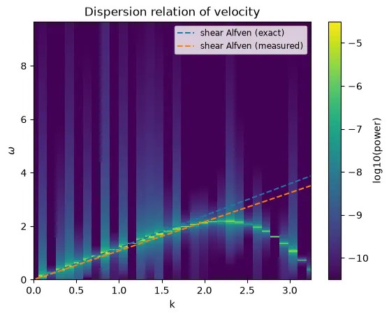
The magnetosonic branches
Section titled “The magnetosonic branches”The same, for the pressure field: both the slow and fast magnetosonic branches appear in one
spectrum, so both get a branches entry. Both track their exact speeds closely below
k ~ 2, where the fit was taken from; above that, both ridges bend away from the straight
omega = v * k line as the real numerical dispersion of the discretization takes over —
an honest feature of the run, not a plotting bug.
    pressure_path = OUT / "real_dispersion_pressure.png"
    pressure_result = pressure.plasma.plot.dispersion(
        branches={
            "slow (exact)": lambda k: exact_speeds["slow magnetosonic"] * k,
            "slow (measured)": lambda k: measured_slow * k,
            "fast (exact)": lambda k: exact_speeds["fast magnetosonic"] * k,
            "fast (measured)": lambda k: measured_fast * k,
        },
        kmax=kmax,
        omega_max=omega_max,
    )
    pressure_result.ax.set_ylim(0, omega_max)
    pressure_result.ax.set_xlim(0, kmax)
    pressure_result.save(pressure_path, close=True)
    print(f"wrote {pressure_path}")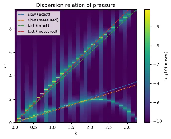
Full script
Section titled “Full script”scripts/generate_real_example_figures.py, unedited
"""Generate the figures for the "MHD slab waves" guide
(docs/src/assets/figures/real_*).

Every other example figure in the docs uses small synthetic data (see
``generate_docs_figures.py``) so contributors can build the docs without a full
struphy install. This script is the one exception: it's a real struphy
simulation, adapted from struphy's own gallery example (mhd-slab-waves), run
right here -- so it needs the full compiled struphy runtime (see
.github/workflows/docs.yml and CONTRIBUTING.md for the system packages and the
`struphy compile` step).

Run from the repo root: python scripts/generate_real_example_figures.py
(or: make figures, which runs this and generate_docs_figures.py)
"""

from __future__ import annotations

import sys
import tempfile
import time
from pathlib import Path

import matplotlib

matplotlib.use("Agg")

import numpy as np

sys.path.insert(0, str(Path(__file__).resolve().parents[1] / "src"))
import plasma_plots  # noqa: F401  (registers .plasma on DataArray/Dataset)

DOCS = Path(__file__).resolve().parents[1] / "docs"
OUT_SIM = DOCS / "src" / "assets" / "simulations"
OUT = DOCS / "src" / "assets" / "figures"
OUT.mkdir(parents=True, exist_ok=True)


# =============================================================================
# A real magnetized slab: struphy.models.LinearMHD, in a uniform, obliquely
# magnetized plasma (struphy.fields_background.equils.HomogenSlab). Broadband
# noise in the velocity excites all three MHD wave branches along z at once:
# the shear Alfvén wave, and the slow and fast magnetosonic waves.
# Adapted from struphy's own gallery example (mhd-slab-waves).
# =============================================================================
from struphy import (
    DerhamOptions,
    EnvironmentOptions,
    Time,
    domains,
    equils,
    grids,
    perturbations,
)
from struphy.models import LinearMHD
from struphy.post_processing.output import Output
from struphy.simulation.sim import Simulation

# The background: B0 = (0, 1, 1), density 0.7, plasma beta 3 (thermal over
# magnetic pressure).
B0x, B0y, B0z = 0.0, 1.0, 1.0
n0, beta, gamma = 0.7, 3.0, 5.0 / 3.0
B_squared = B0x**2 + B0y**2 + B0z**2
p0 = beta * B_squared / 2.0

# The exact ideal-MHD wave speeds along z, to compare the measured ones
# against.
alfven_speed = np.sqrt(B_squared / n0)
sound_speed = np.sqrt(gamma * p0 / n0)
cs2, va2 = sound_speed**2, alfven_speed**2
delta = 4 * B0z**2 * cs2 * va2 / ((cs2 + va2) ** 2 * B_squared)
exact_speeds = {
    "shear Alfven": alfven_speed * B0z / np.sqrt(B_squared),
    "slow magnetosonic": np.sqrt(0.5 * (cs2 + va2) * (1 - np.sqrt(1 - delta))),
    "fast magnetosonic": np.sqrt(0.5 * (cs2 + va2) * (1 + np.sqrt(1 - delta))),
}


def run_simulation() -> Output:

    model = LinearMHD()
    model.propagators.shear_alf.options = model.propagators.shear_alf.Options(
        algo="implicit"
    )
    for component in range(3):
        model.mhd.velocity.add_perturbation(
            perturbations.Noise(amp=0.1, comp=component, seed=123)
        )
    equil = equils.HomogenSlab(B0x=B0x, B0y=B0y, B0z=B0z, beta=beta, n0=n0)

    sim = Simulation(
        model=model,
        env=EnvironmentOptions(sim_folder="mhd_slab_waves"),
        time_opts=Time(dt=0.15, Tend=180.0),
        domain=domains.Cuboid(r3=60.0),
        grid=grids.TensorProductGrid(num_elements=(1, 1, 64)),
        derham_opts=DerhamOptions(degree=(1, 1, 3)),
        equil=equil,
    )
    out = sim.run()
    return out


def pproc(out: Output):
    # Both fields are evaluated at a single (eta1, eta2) point, physical z as
    # the remaining spatial coordinate (logical eta3 swapped for physical Z, so
    # k comes out in physical units, matching the exact speeds above).
    velocity = out.evaluate("mhd/velocity", component=0).isel(eta1=0, eta2=0)
    velocity = velocity.assign_coords(eta3=("eta3", velocity["Z"].values))
    pressure = out.evaluate("mhd/pressure").isel(eta1=0, eta2=0)
    pressure = pressure.assign_coords(eta3=("eta3", pressure["Z"].values))

    velocity_spectrum = velocity.plasma.analysis.dispersion(dim="eta3")
    pressure_spectrum = pressure.plasma.analysis.dispersion(dim="eta3")

    fit_k_range = (0.2, 2.0)
    (alfven_branch,) = velocity_spectrum.plasma.analysis.fit_branches(
        n_branches=1, k_range=fit_k_range, noise_level=0.5
    )
    # The fast branch's power is only a few percent of the slow branch's peak
    # power in this window, so noise_level has to be low enough to still count
    # it as a genuine peak.
    slow_branch, fast_branch = pressure_spectrum.plasma.analysis.fit_branches(
        n_branches=2, k_range=fit_k_range, noise_level=0.02
    )
    measured_alfven, measured_slow, measured_fast = (
        alfven_branch.velocity,
        slow_branch.velocity,
        fast_branch.velocity,
    )
    measured_speeds = {
        "shear Alfven": measured_alfven,
        "slow magnetosonic": measured_slow,
        "fast magnetosonic": measured_fast,
    }
    for branch, exact in exact_speeds.items():
        measured = measured_speeds[branch]
        print(f"{branch}: measured {measured:.4f}, exact {exact:.4f}")

    # Show the whole resolved spectrum
    k_top = min(
        float(velocity_spectrum.k.max()), float(pressure_spectrum.k.max())
    )
    omega_nyquist = min(
        float(velocity_spectrum.omega.max()),
        float(pressure_spectrum.omega.max()),
    )
    kmax = k_top
    omega_max = min(exact_speeds["fast magnetosonic"] * k_top, omega_nyquist)

    velocity_path = OUT / "real_dispersion_velocity.png"
    velocity_result = velocity.plasma.plot.dispersion(
        branches={
            "shear Alfven (exact)": lambda k: exact_speeds["shear Alfven"] * k,
            "shear Alfven (measured)": lambda k: measured_alfven * k,
        },
        kmax=kmax,
        omega_max=omega_max,
    )

    velocity_result.ax.set_ylim(0, omega_max)
    velocity_result.ax.set_xlim(0, kmax)
    velocity_result.save(velocity_path, close=True)
    print(f"wrote {velocity_path}")

    pressure_path = OUT / "real_dispersion_pressure.png"
    pressure_result = pressure.plasma.plot.dispersion(
        branches={
            "slow (exact)": lambda k: exact_speeds["slow magnetosonic"] * k,
            "slow (measured)": lambda k: measured_slow * k,
            "fast (exact)": lambda k: exact_speeds["fast magnetosonic"] * k,
            "fast (measured)": lambda k: measured_fast * k,
        },
        kmax=kmax,
        omega_max=omega_max,
    )
    pressure_result.ax.set_ylim(0, omega_max)
    pressure_result.ax.set_xlim(0, kmax)
    pressure_result.save(pressure_path, close=True)
    print(f"wrote {pressure_path}")


if __name__ == "__main__":
    import argparse

    argparser = argparse.ArgumentParser(
        description="Run the mhd slab waves example."
    )
    argparser.add_argument(
        "--pproc-only",
        action="store_true",
        help="Post-process an existing run instead of running a new one.",
    )
    args = argparser.parse_args()

    if not args.pproc_only:
        out = run_simulation()
    else:
        out = Output("mhd_slab_waves")

    pproc(out)

print("done")
More examples
Section titled “More examples”This is one of many. The Struphy examples gallery has 48 more, covering every physics module — a few to start with:
- Shear-Alfvén wave dispersion — the same kind of measurement as this page, for the simplest case.
- Whistler and ion-cyclotron waves in Hall MHD — the same idea, extended to non-linear branches.
- Orszag–Tang vortex — a standard nonlinear MHD benchmark.
- Two-stream instability — kinetic, not fluid.
- Guiding-center orbits in a tokamak — particle orbits rather than fields.