Theory toolbox
plasma_plots.theory collects the analytic results that Struphy runs are
checked against: dispersion relations and growth rates, plasma parameters,
particle orbits, exact solutions, and the properties of the numerics
themselves. It is plain numpy, needs neither Struphy nor scipy, and its
results plug straight into the plots.
from plasma_plots.theory import ( exact, kinetic, numerics, orbits, parameters, waves,)Full signatures are in the theory reference.
Conventions
Section titled “Conventions”- Arrays: every function takes scalars or numpy arrays that broadcast, and returns arrays (a Python scalar for scalar input).
- Units: normalized, unless a function says otherwise. Kinetic results use
the plasma frequency, the Debye length and v_th = √(T/m). Fluid and MHD
results come out in the units of the speeds and wavenumbers you pass.
theory.parametersis in SI units, with temperatures in eV. - Frequencies are complex, for
exp(i(k·x − ωt)): the real part is the frequency, a positive imaginary part a growth rate, a negative one a damping rate. Take.realor.imagto plot one of them. - Several branches come as a dict of names to complex frequencies, e.g.
{"shear Alfvén": ..., "slow": ..., "fast": ...}.
Using theory with the plots
Section titled “Using theory with the plots”A theory function goes directly into the plots that compare against theory:
phi.plasma.plot.dispersion(    branches={"kinetic": kinetic.langmuir, "Bohm–Gross": kinetic.bohm_gross})v.plasma.plot.dispersion(    branches=lambda k: waves.mhd_waves(        k, theta=0.3, alfven_speed=1.0, sound_speed=0.5    ))
spectrum = phi.plasma.analysis.dispersion()# follow the kinetic branchtraced = spectrum.plasma.analysis.trace_branch(kinetic.langmuir)# frequencies and their errorstraced.omega.plasma.plot.against_theory(kinetic.langmuir)# damping ratesrates.plasma.plot.against_theory(lambda k: kinetic.langmuir(k).imag)
T.plasma.plot.profiles( x="eta1", reference=lambda x, t: exact.heat_kernel( x, t, 0.01, width=0.05, center=0.5 ),)branches=takes a dict of labels to functions, or one function that returns a dict of branches. Complex frequencies are drawn by their real part.- Struphy’s own
struphy.dispersion_relationsobjects, such asMHDhomogenSlab(), work asbranches=too. trace_branchandagainst_theorycompare frequencies (the real part). For growth or damping rates, pass the imaginary part.
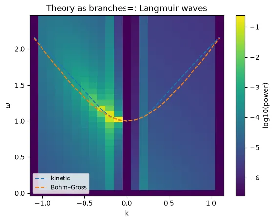
A synthetic field of damped Langmuir waves, with the kinetic root and Bohm–Gross drawn over its spectrum. The kinetic curve follows the measured ridge where Bohm–Gross drifts away:
Kinetic waves and instabilities
Section titled “Kinetic waves and instabilities”theory.kinetic solves the electrostatic dispersion relation of drifting
Maxwellians with the plasma dispersion function Z(ζ). It covers Langmuir waves
with their Landau damping, ion-acoustic waves, and the beam-driven
instabilities, plus the electromagnetic Weibel instability:
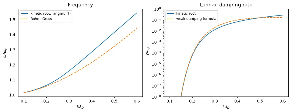
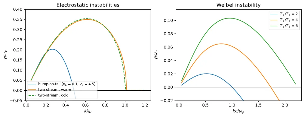
kinetic.langmuir(0.5) # (1.415662−0.153359j): frequency and Landau dampingkinetic.ion_acoustic(k, temperature_ratio=10)kinetic.bump_on_tail( k, beam_density=0.1, beam_speed=4.5, beam_thermal_speed=0.5)kinetic.two_stream(k, beam_speed=1.0, thermal_speed=0.1)kinetic.weibel(k, anisotropy=4.0, parallel_thermal_speed=0.1) # k in ω_p/c# (k, ω) of the fastest growthkinetic.maximum_growth(kinetic.bump_on_tail, (0.05, 0.5))For other velocity distributions, describe each species as a
kinetic.Maxwellian(density, charge, mass, thermal_speed, drift), and solve
kinetic.electrostatic_dielectric(ω, k, species) = 0 with
kinetic.solve_dispersion.
Fluid, MHD and cold-plasma waves
Section titled “Fluid, MHD and cold-plasma waves”theory.waves covers the linear waves of Struphy’s fluid and field models:
| Function | Model |
|---|---|
light_wave, plasma_light_wave, cavity_modes |
Maxwell, a cavity, the O-wave cutoff |
mhd_waves, magnetosonic_speeds |
ideal MHD at any angle |
dissipative_alfven |
resistive and viscous MHD |
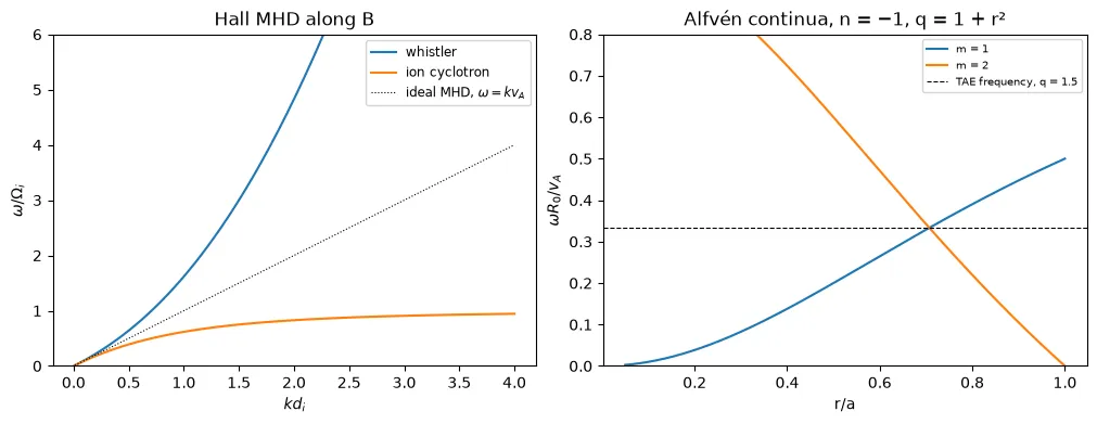
hall_mhd_parallel |
Hall MHD along B: whistler and ion-cyclotron waves |
stix, refractive_index, cold_plasma_waves, appleton_hartree, cutoffs, resonances, faraday_rotation |
cold plasma |
drift_wave, hasegawa_wakatani |
drift waves |
alfven_continuum, slow_continuum, tae_frequency |
continuous spectra and the TAE frequency |
# {"shear Alfvén", "slow", "fast"}waves.mhd_waves(k, theta=np.pi / 4, alfven_speed=1.0, sound_speed=0.6)plasma = waves.electron_ion( plasma_frequency=1.0, cyclotron_frequency=0.6, mass_ratio=25)waves.cold_plasma_waves(k, np.pi / 4, plasma) # every branch at 45°waves.cutoffs(plasma), waves.resonances(np.pi / 4, plasma)waves.faraday_rotation(omega, length, plasma)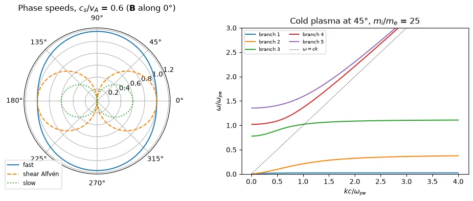
The continua follow Struphy’s MhdContinousSpectraCylinder:
k∥ = (n + m/q)/R₀. The m and m + 1 continua cross at q = −(m + ½)/n, e.g.
q = 1.5 for m = 1, n = −1, at the TAE frequency v_A/(2qR₀). In a torus the
toroidal coupling of the two harmonics opens a gap there, where toroidal Alfvén
eigenmodes live. The
continuous-spectrum plot
draws the continua over a measured spectrum.
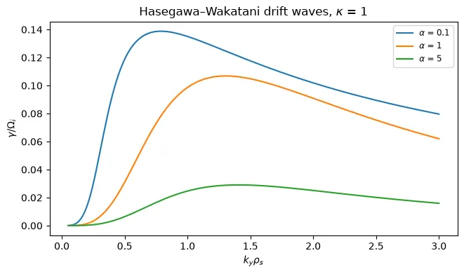
hasegawa_wakatani solves the standard linear Hasegawa–Wakatani equations,
∂(∇²φ)/∂t = α(φ − n) and ∂n/∂t = α(φ − n) − κ ∂φ/∂y, with lengths in ρ_s and
time in 1/Ω_i. Check the sign convention against your model before comparing
growth rates.
Plasma parameters and Struphy’s units
Section titled “Plasma parameters and Struphy’s units”theory.parameters gives the standard plasma frequencies, lengths, speeds and
dimensionless numbers in SI units, checked against the NRL
Plasma Formulary. It also gives the units Struphy normalizes with:
parameters.alfven_speed(field=1.0, density=1e20, mass_number=2) # m/sparameters.debye_length(density=1e19, temperature=100.0) # m, T in eVunits = parameters.struphy_units( x=1.0, B=1.0, n=1.0, velocity_scale="alfvén", mass_number=1)units["t"], units["v"] # Struphy's time and velocity units# α, ε, κ of a speciesparameters.struphy_equation_parameters(units, charge_number=1, mass_number=1)struphy_units takes the same arguments as Struphy’s BaseUnits and mirrors
Units.derive_units, so normalized results can be converted to physical ones
and back.
Particle orbits
Section titled “Particle orbits”theory.orbits has the gyromotion, the E×B and grad-B drifts as 3-vectors,
and trapped particles in a
large-aspect-ratio tokamak with B = B₀/(1 + ε cos θ). That covers the trapped
fraction, the trapped–passing boundary, bounce and transit frequencies, and
banana widths:
orbits.gyroradius(perpendicular_speed=1.0, field=1.0)# B, grad_B: arrays with a last axis of 3orbits.grad_b_drift(1.0, B, grad_B, charge=1.0, mass=1.0)orbits.trapped_fraction(0.3)kappa2 = orbits.trapping_parameter( orbits.pitch_parameter(0.2, epsilon=0.1), epsilon=0.1)orbits.bounce_frequency( 1.0, kappa2, epsilon=0.1, safety_factor=2.0, major_radius=3.0)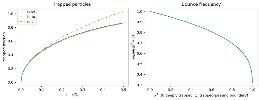
Exact solutions
Section titled “Exact solutions”theory.exact has exact solutions to verify runs. Most take (x, t) first, so
they work as reference= of the profile plots:
| Function | Solution |
|---|---|
riemann_euler, sod_shock_tube, star_state |
the Euler Riemann problem, including vacuum |
dam_break |
Ritter’s dam break on a dry bed |
heat_kernel |
diffusion (also of a magnetic field, or of momentum by viscosity) |
advected, dalembert |
advection and waves |
pressureless, pressureless_eulerian, caustic_time |
pressureless flow and its caustics (Zel’dovich) |
sod = exact.sod_shock_tube(x, 0.2) # .density, .velocity, .pressurerho.plasma.plot.lineout( x="eta1", t=-1, reference=lambda x, t: exact.sod_shock_tube(x, t).density)exact.caustic_time(lambda q: -0.5 * np.sin(q), q) # first shell crossing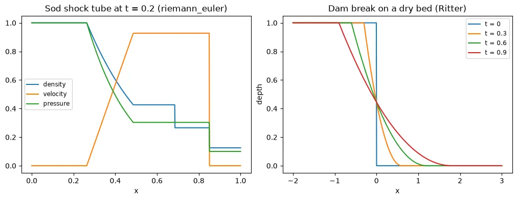
Properties of the numerics
Section titled “Properties of the numerics”theory.numerics tells what errors the numerics themselves produce, so a
measured drift or frequency error can be judged:
- the amplification factor, amplitude and phase errors and stability limits of time integrators (explicit and implicit Euler, implicit midpoint, Störmer–Verlet, RK2–RK4)
- the numerical dispersion of B-spline Galerkin finite elements, as in Struphy’s discrete de Rham complex
numerics.phase_error(omega * dt, "implicit_midpoint") # ≈ −(ωΔt)²/12# the complex frequency the scheme producesnumerics.numerical_frequency(omega, dt, "rk4")numerics.stability_limit("rk4") # the largest stable ωΔt, 2√2# ω of the discrete wave equationnumerics.spline_galerkin_dispersion(k, dx, degree=3)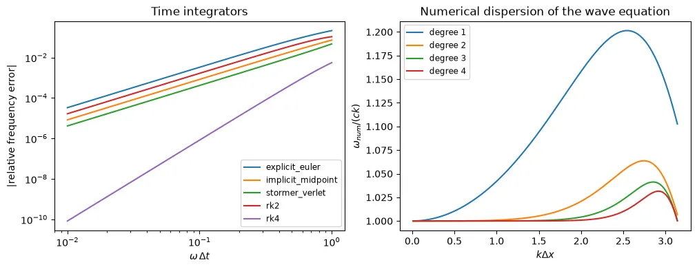
Which tool for which Struphy example
Section titled “Which tool for which Struphy example”The Struphy examples and the analytic results to compare them with:
| Examples | Theory |
|---|---|
| Langmuir wave dispersion, weak and strong Landau damping | kinetic.langmuir, bohm_gross, landau_damping_weak |
| Two-stream and bump-on-tail instabilities | kinetic.two_stream, two_stream_cold, bump_on_tail, maximum_growth |
| Weibel instability | kinetic.weibel |
| Maxwell light-wave dispersion, cavity resonances | waves.light_wave, cavity_modes |
| Cold-plasma oscillation, wave packets, waves along a magnetic field | waves.cold_plasma_waves, stix, group_velocity |
| Ordinary waves and the plasma cutoff, Faraday rotation | waves.plasma_light_wave, cutoffs, faraday_rotation |
| MHD waves in a slab, shear-Alfvén dispersion, standing shear-Alfvén wave | waves.mhd_waves, magnetosonic_speeds |
| Resistively damped, viscous and resistive Alfvén waves | waves.dissipative_alfven |
| Whistler and ion-cyclotron waves in Hall MHD | waves.hall_mhd_parallel |
| Toroidal shear-Alfvén waves | waves.alfven_continuum, tae_frequency |
| Hasegawa–Wakatani drift-wave turbulence | waves.hasegawa_wakatani, drift_wave |
| Gyromotion, grad-B drift | orbits.gyrofrequency, gyroradius, grad_b_drift |
| Guiding-center and Vlasov orbits in a tokamak | orbits.trapped_fraction, bounce_frequency, transit_frequency, banana_width |
| Resistive diffusion of a magnetic field | exact.heat_kernel (a mode decays as exp(−ηk²t)) |
| Acoustic pulse | exact.dalembert |
| Gas expansion into vacuum | exact.riemann_euler (with a vacuum state) |
| Dam break | exact.dam_break |
| Zel’dovich caustic, pressureless density transport | exact.pressureless, caustic_time, advected |
| Random and deterministic particle diffusion, SPH velocity diffusion | exact.heat_kernel (spread 2Dt) |
| Incompressible shear relaxation | exact.heat_kernel (a shear mode decays as exp(−νk²t)) |
| Structure preservation in time integration | numerics.amplification_factor, phase_error, numerical_frequency |
| Every run: physical units | parameters.struphy_units |