DESC equilibria
DESC computes 3-D MHD equilibria and evaluates any of several
hundred quantities of them on a grid of flux coordinates, eq.compute(names, grid), as flat
arrays over the grid’s nodes. plasma_plots.from_desc evaluates an equilibrium on a grid and
returns an xarray.Dataset in the layout the rest of plasma-plots reads, the same as for
GVEC:
import desc.examplesimport plasma_plots
w7x = desc.examples.get("W7-X")  # or desc.io.load("path/to/eq.h5")ev = plasma_plots.from_desc(    w7x,    ["|B|", "iota", "p", "sqrt(g)", "D_Mercier", "theta_PEST"],    rho=17,    theta=64,    zeta=40,)ev["|B|"].plasma.plot.slice(coords="physical", plane="RZ", zeta=0.0)
Every figure on this page comes from the equilibria that DESC ships with (desc.examples), made
while the docs are built (scripts/generate_desc_figures.py, at the end of the page). Evaluating
needs DESC (pip install desc-opt, or pip install "plasma-plots[desc]"); the Dataset it returns
does not, and ev.to_netcdf("w7x.nc") saves it for plotting elsewhere.
Reading DESC’s quantities
Section titled “Reading DESC’s quantities”rho, theta and zeta each take a number of points (spread over [0, 1], [0, 2π) and one
field period [0, 2π/nfp)) or the values themselves, which may cover the whole torus. What
from_desc makes of DESC’s output:
| DESC | plasma-plots |
|---|---|
| flat arrays over the grid’s nodes | dimensions rho, theta, zeta: select with rho=0.5, draw with x="zeta" |
"X", "Y", "Z" |
the coordinates X, Y, Z of every variable: coords="physical", plane="RZ", 3-D views, gradients |
vectors ("B", "J", …) in cylindrical (R, φ, Z) components |
Cartesian components along component, as for Struphy’s and GVEC’s vectors |
profiles ("iota", "p", "D_Mercier") and global quantities ("V") |
variables over rho alone, and scalars |
"theta_PEST" |
the coordinate theta_P, for lines of constant PEST angle |
label, units, description of DESC’s list of variables |
label ($\iota$), units and long_name, for axes and color bars |
eq.NFP |
the nfp attribute; the angles get a period (2π, 2π/nfp) |
The variables keep DESC’s names, so ev["|B|"] and ev["sqrt(g)"] (DESC’s Jacobian); names
that are identifiers also work as attributes, ev.iota. sfl="pest" evaluates on a grid in the
PEST angle instead, over (rho, theta_P, zeta); DESC finds its own theta of each point with
eq.map_coordinates, and it becomes a coordinate.
Poloidal planes
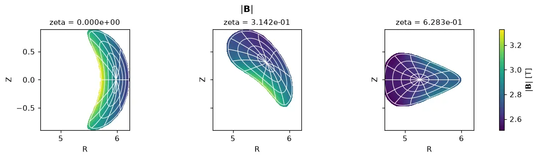
Section titled “Poloidal planes”planes = plasma_plots.from_desc( w7x, ["|B|", "theta_PEST"], rho=13, theta=96, zeta=np.linspace(0, np.pi / w7x.NFP, 3),)planes["|B|"].plasma.plot.panels( sweep="zeta", coords="physical", plane="RZ", nrows=1, ncols=3, overlays={"coordinate_lines": {"rho": 4, "theta_P": 12}},)W7-X over half a field period, from the bean-shaped plane at zeta = 0 to the triangular one,
with four flux surfaces and twelve lines of constant PEST angle. coordinate_lines draws lines of
constant value of either drawn dimension ({"rho": 4, "theta": 8} for DESC’s own angle), or
contour lines of another coordinate over them, here theta_P.
The same plot with Plotly
One plane, with backend="plotly" (see Interactive plots with Plotly).
ev["|B|"].plasma.plot.slice( coords="physical", plane="RZ", zeta=0.0, overlays={"coordinate_lines": {"rho": 4, "theta_P": 12}}, backend="plotly",)Loading interactive chart…
DESC’s examples side by side, each at zeta = 0, in one figure with
plasma_plots.figure:
gallery = ["precise_QA", "precise_QH", "NCSX", "HELIOTRON", "ESTELL", "DSHAPE"]with plasma_plots.figure(2, 3, figsize=(12, 8)) as fig: for ax, name in zip(fig, gallery): plane = plasma_plots.from_desc( desc.examples.get(name), ["|B|", "theta_PEST"], rho=9, theta=64, zeta=[0.0], ) plane["|B|"].plasma.plot.slice( coords="physical", plane="RZ", zeta=0.0, title=name, overlays={"coordinate_lines": {"rho": 4, "theta_P": 8}}, ax=ax, )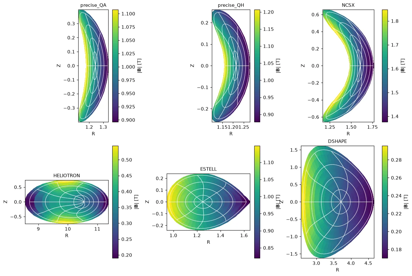
On a flux surface
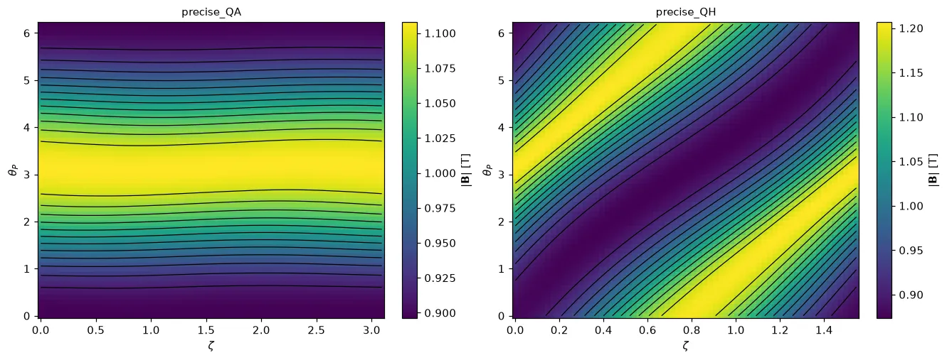
Section titled “On a flux surface”qa, qh = desc.examples.get("precise_QA"), desc.examples.get("precise_QH")surfaces = { name: plasma_plots.from_desc( eq, "|B|", rho=[0.5, 1.0], theta=64, zeta=64, sfl="pest" ) for name, eq in (("precise_QA", qa), ("precise_QH", qh))}with plasma_plots.figure(1, 2, figsize=(12, 4.5)) as fig: for ax, (name, surface) in zip(fig, surfaces.items()): surface["|B|"].plasma.plot.slice( x="zeta", y="theta_P", rho=1.0, levels=12, title=name, ax=ax )|B| on the last flux surface of the precise quasi-axisymmetric (left) and quasi-helically
symmetric (right) stellarators, over one field period in the PEST angle: its contours run almost
straight in the toroidal and in the helical direction. levels=12 adds the contour lines.
Quasi-symmetry is a property of |B| in Boozer angles; in the PEST angle, as here, the contours are
close to straight but not exactly.
The same plot with Plotly
surfaces["precise_QH"]["|B|"].plasma.plot.slice( x="zeta", y="theta_P", rho=1.0, levels=12, backend="plotly")Loading interactive chart…
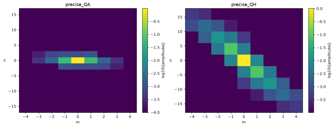
The same surfaces as Fourier amplitudes over poloidal m and toroidal n:
for name, surface in surfaces.items(): surface["|B|"].plasma.plot.mode_map( rho=1.0, m_range=(-4, 4), n_range=(-16, 16) )The transform takes the angles’ periods from the Dataset, so n is the full-torus mode number, a
multiple of nfp (2 for precise_QA, 4 for precise_QH). The quasi-axisymmetric spectrum sits on
n = 0, the quasi-helical one on the line n = -nfp · m. See
Spectral analysis for the other mode tools, e.g.
mode_spectrum() for the complex amplitudes.
Profiles
Section titled “Profiles”from plasma_plots.analysis import surface_average
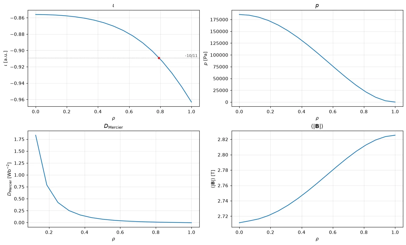
with plasma_plots.figure(2, 2) as fig: ev.iota.plasma.plot.lineout(rationals=4, ax=fig[0]) ev.p.plasma.plot.lineout(ax=fig[1]) # singular on the axis ev.D_Mercier.sel(rho=slice(0.1, None)).plasma.plot.lineout(ax=fig[2]) ev["|B|"].plasma.analysis.surface_average( jacobian=ev["sqrt(g)"] ).plasma.plot.lineout(ax=fig[3])W7-X’s rotational transform, pressure, Mercier criterion (positive where stable) and flux-surface
average of |B|. DESC’s ι of W7-X is negative, a matter of the equilibrium’s orientation; the
rational surfaces keep the sign, -10/11. rationals=4 marks the lowest-order rational values n/m of
ι that the profile reaches, with n a multiple of nfp, and
ev.iota.plasma.analysis.rational_surfaces(count=4) returns them. surface_average is
⟨f⟩ = ∫ f √g dθ dζ / ∫ √g dθ dζ, with DESC’s Jacobian "sqrt(g)".
The same plot with Plotly
ev.iota.plasma.plot.lineout(rationals=4, backend="plotly")Loading interactive chart…
For a tokamak, DESC’s DSHAPE, the safety factor q = 1/ι works the same way:
dshape = desc.examples.get("DSHAPE")tok = plasma_plots.from_desc( dshape, ["|B|", "iota", "theta_PEST"], rho=17, theta=64, zeta=[0.0])q = (1 / tok.iota).rename("q")q.attrs = {"label": "$q$", "nfp": 1}with plasma_plots.figure(1, 2) as fig: tok["|B|"].plasma.plot.slice( coords="physical", plane="RZ", zeta=0.0, overlays={"coordinate_lines": {"rho": 5, "theta_P": 12}}, ax=fig[0], ) q.plasma.plot.lineout(rationals=4, ax=fig[1])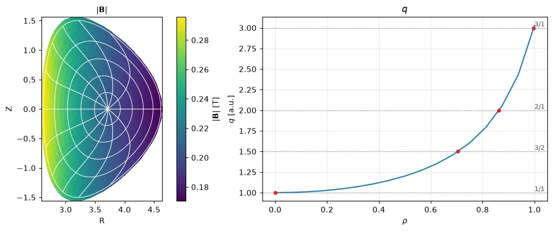
Currents
Section titled “Currents”Any of DESC’s quantities over the grid draws the same way, e.g. the magnitude of the current density in W7-X’s bean-shaped plane:
fields = plasma_plots.from_desc( w7x, ["|J|", "theta_PEST"], rho=np.linspace(0.05, 1, 20), theta=64, zeta=24)fields["|J|"].plasma.plot.slice( coords="physical", plane="RZ", zeta=0.0, overlays={"coordinate_lines": {"rho": 4, "theta_P": 12}},)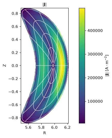
The vectors ("J", "B", "grad(|B|)", …) come in Cartesian components: with "J" among
the names, fields.J.sel(component="z") is the vertical current density, and plasma-plots’ vector calculus on the
mapped domain (.plasma.analysis.divergence(), .curl(), see
Diagnostics) applies to them as to any other.
Integrals
Section titled “Integrals”import xarray as xrfrom plasma_plots.analysis import volume_integral
fine = plasma_plots.from_desc( w7x, ["|B|", "sqrt(g)", "V"], rho=33, theta=64, zeta=48)volume = ( volume_integral(xr.ones_like(fine["sqrt(g)"]), jacobian=fine["sqrt(g)"]) * w7x.NFP)volume_integral integrates over the sampled grid, one field period here, so multiply by nfp
for the whole device. On the uniform grid the angles get the rectangle rule, which is exact for
their Fourier modes, and the radius the trapezoidal rule. jacobian= takes DESC’s "sqrt(g)";
without it, √g comes from the geometry. For W7-X, against DESC’s own numbers:
W7-X volume, DESC's own V                        27.8479632616
volume_integral(1, jacobian=sqrt(g)) * nfp       27.8476442507
volume_integral(1) * nfp, sqrt(g) from X, Y, Z   27.8472616121
<|B|> at rho = 0.5, DESC's own                   2.7629138923
surface_average(|B|, jacobian=sqrt(g))           2.7629138924
In 3-D
Section titled “In 3-D”With PyVista (see 3-D views), on a grid over the whole torus
(every field period). cuts take rho, theta and zeta like Struphy’s eta1, eta2, eta3.
precise_QH’s last flux surface, all four field periods:
qh_torus = plasma_plots.from_desc( qh, "|B|", rho=[1.0], theta=64, zeta=np.linspace(0, 2 * np.pi, 32 * qh.NFP, endpoint=False),)qh_torus["|B|"].plasma.plot.slices_3d().show()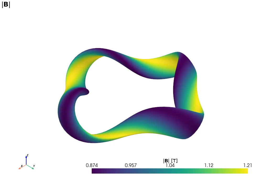
Drag to rotate, scroll to zoom, shift-drag to pan.Open in a new tab
W7-X, with an inner surface and three poloidal cuts inside the translucent outer surface:
torus = plasma_plots.from_desc( w7x, ["|B|", "B"], rho=9, theta=48, zeta=np.linspace(0, 2 * np.pi, 32 * w7x.NFP, endpoint=False),)torus["|B|"].plasma.plot.slices_3d( cuts={"rho": [0.5], "zeta": [0.0, np.pi / 2, np.pi]}).show()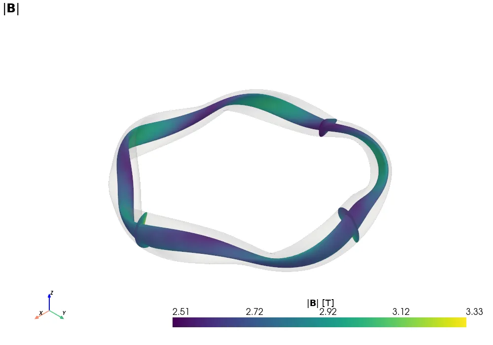
Drag to rotate, scroll to zoom, shift-drag to pan.Open in a new tab
Magnetic field lines, traced through DESC’s B from a small sphere of seeds next to the axis:
axis = torus.isel(rho=0, theta=0, zeta=0)torus.B.plasma.plot.streamlines( n_points=40, source_center=(float(axis.X) + 0.2, float(axis.Y), float(axis.Z)), source_radius=0.15, tube_radius=0.02,).show()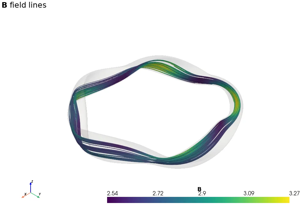
Drag to rotate, scroll to zoom, shift-drag to pan.Open in a new tab
The script behind this page
Section titled “The script behind this page”It loads DESC’s examples, evaluates them and writes every figure above, in about two minutes.
scripts/generate_desc_figures.py, unedited
"""Generate the figures of the "DESC equilibria" guide
(docs/src/assets/figures/desc_*) from real DESC equilibria.

Like ``generate_gvec_figures.py`` for GVEC, this uses the actual code: the
example equilibria that DESC ships (W7-X, the precise quasi-axisymmetric and
quasi-helical stellarators, NCSX, HELIOTRON, ESTELL and the tokamak DSHAPE),
evaluated with ``plasma_plots.from_desc`` and plotted with plasma-plots. It
needs ``pip install desc-opt`` (pure Python, on JAX); the interactive 3-D
scenes need PyVista and trame-pyvista, the Plotly charts plotly (see
.github/workflows/docs.yml).

Run from the repo root: python scripts/generate_desc_figures.py (or: make
figures).
"""

from __future__ import annotations

import sys
import warnings
from pathlib import Path

import matplotlib

matplotlib.use("Agg")

import desc.examples
import matplotlib.pyplot as plt
import numpy as np
import xarray as xr
from desc.grid import LinearGrid

sys.path.insert(0, str(Path(__file__).resolve().parents[1] / "src"))
import plasma_plots
from plasma_plots.analysis import surface_average, volume_integral

# DESC's notes on JAX, grids and resolutions
warnings.filterwarnings("ignore", module="desc")

ROOT = Path(__file__).resolve().parents[1]
DOCS = ROOT / "docs"
OUT = DOCS / "src" / "assets" / "figures"
NUMBERS = DOCS / "src" / "assets" / "desc" / "numbers.txt"
PLOTLY_OUT = DOCS / "public" / "plotly"
PYVISTA_OUT = DOCS / "public" / "pyvista"
for folder in (OUT, NUMBERS.parent, PLOTLY_OUT, PYVISTA_OUT):
    folder.mkdir(parents=True, exist_ok=True)


def save(result, filename):
    result.save(OUT / filename, close=True)
    print(f"wrote {OUT / filename}")


def save_plotly(result, filename):
    print(f"wrote {result.save(PLOTLY_OUT / f'{filename}.json')}")


def example(name):
    with warnings.catch_warnings():
        warnings.simplefilter("ignore")
        return desc.examples.get(name)


# =============================================================================
# W7-X: one field period on DESC's angles, with the PEST angle for coordinate
# lines
# =============================================================================
w7x = example("W7-X")
ev = plasma_plots.from_desc(
    w7x,
    ["|B|", "iota", "p", "sqrt(g)", "D_Mercier", "theta_PEST"],
    rho=17,
    theta=64,
    zeta=40,
)
lines = {"coordinate_lines": {"rho": 4, "theta_P": 12}}

# =============================================================================
# Poloidal planes: W7-X over half a field period, and DESC's example library at
# zeta = 0
# =============================================================================
planes = plasma_plots.from_desc(
    w7x,
    ["|B|", "theta_PEST"],
    rho=13,
    theta=96,
    zeta=np.linspace(0, np.pi / w7x.NFP, 3),
)
save(
    planes["|B|"].plasma.plot.panels(
        sweep="zeta",
        coords="physical",
        plane="RZ",
        nrows=1,
        ncols=3,
        overlays=lines,
    ),
    "desc_w7x_planes.png",
)

gallery = ["precise_QA", "precise_QH", "NCSX", "HELIOTRON", "ESTELL", "DSHAPE"]
with plasma_plots.figure(2, 3, figsize=(12, 8)) as fig:
    for ax, name in zip(fig, gallery):
        plane = plasma_plots.from_desc(
            example(name), ["|B|", "theta_PEST"], rho=9, theta=64, zeta=[0.0]
        )
        plane["|B|"].plasma.plot.slice(
            coords="physical",
            plane="RZ",
            zeta=0.0,
            title=name,
            overlays={"coordinate_lines": {"rho": 4, "theta_P": 8}},
            ax=ax,
        )
save(fig, "desc_gallery.png")

# =============================================================================
# On a flux surface: quasi-axisymmetry and quasi-helical symmetry, in PEST
# angles
# =============================================================================
qa, qh = example("precise_QA"), example("precise_QH")
surfaces = {
    name: plasma_plots.from_desc(
        eq, "|B|", rho=[0.5, 1.0], theta=64, zeta=64, sfl="pest"
    )
    for name, eq in (("precise_QA", qa), ("precise_QH", qh))
}
with plasma_plots.figure(1, 2, figsize=(12, 4.5)) as fig:
    for ax, (name, surface) in zip(fig, surfaces.items()):
        surface["|B|"].plasma.plot.slice(
            x="zeta", y="theta_P", rho=1.0, levels=12, title=name, ax=ax
        )
save(fig, "desc_surfaces.png")
with plasma_plots.figure(1, 2, figsize=(12, 4.5)) as fig:
    for ax, (name, surface) in zip(fig, surfaces.items()):
        surface["|B|"].plasma.plot.mode_map(
            rho=1.0, m_range=(-4, 4), n_range=(-16, 16), ax=ax
        ).ax.set_title(name)
save(fig, "desc_mode_maps.png")

# =============================================================================
# Profiles: W7-X's rotational transform, pressure, Mercier criterion and <|B|>;
# a tokamak's q
# =============================================================================
with plasma_plots.figure(2, 2) as fig:
    ev.iota.plasma.plot.lineout(rationals=4, ax=fig[0])
    ev.p.plasma.plot.lineout(ax=fig[1])
    # singular on the axis
    ev.D_Mercier.sel(rho=slice(0.1, None)).plasma.plot.lineout(ax=fig[2])
    ev["|B|"].plasma.analysis.surface_average(
        jacobian=ev["sqrt(g)"]
    ).plasma.plot.lineout(ax=fig[3])
save(fig, "desc_profiles.png")

dshape = example("DSHAPE")
tok = plasma_plots.from_desc(
    dshape, ["|B|", "iota", "theta_PEST"], rho=17, theta=64, zeta=[0.0]
)
q = (1 / tok.iota).rename("q")
q.attrs = {"label": "$q$", "nfp": 1}
with plasma_plots.figure(1, 2) as fig:
    tok["|B|"].plasma.plot.slice(
        coords="physical",
        plane="RZ",
        zeta=0.0,
        overlays={"coordinate_lines": {"rho": 5, "theta_P": 12}},
        ax=fig[0],
    )
    q.plasma.plot.lineout(rationals=4, ax=fig[1])
save(fig, "desc_tokamak.png")

# =============================================================================
# Fields: the current density in W7-X's bean-shaped plane
# =============================================================================
fields = plasma_plots.from_desc(
    w7x, ["|J|", "theta_PEST"], rho=np.linspace(0.05, 1, 20), theta=64, zeta=24
)
save(
    fields["|J|"].plasma.plot.slice(
        coords="physical", plane="RZ", zeta=0.0, overlays=lines
    ),
    "desc_current.png",
)

# =============================================================================
# Numbers: plasma-plots' integrals against DESC's own
# =============================================================================
fine = plasma_plots.from_desc(
    w7x, ["|B|", "sqrt(g)", "V"], rho=33, theta=64, zeta=48
)
volume = (
    float(
        volume_integral(
            xr.ones_like(fine["sqrt(g)"]), jacobian=fine["sqrt(g)"]
        )
    )
    * w7x.NFP
)
numerical = float(volume_integral(xr.ones_like(fine["|B|"]))) * w7x.NFP
average = float(
    surface_average(
        fine["|B|"].sel(rho=[0.5]), jacobian=fine["sqrt(g)"].sel(rho=[0.5])
    ).squeeze()
)
desc_average = w7x.compute(
    "<|B|>", grid=LinearGrid(rho=np.array([0.5]), M=32, N=24, NFP=w7x.NFP)
)["<|B|>"][0]
rows = [  # on 33 x 64 x 48 points
    ("W7-X volume, DESC's own V", float(fine.V)),
    ("volume_integral(1, jacobian=sqrt(g)) * nfp", volume),
    ("volume_integral(1) * nfp, sqrt(g) from X, Y, Z", numerical),
    ("<|B|> at rho = 0.5, DESC's own", desc_average),
    ("surface_average(|B|, jacobian=sqrt(g))", average),
]
NUMBERS.write_text(
    "".join(f"{label:<48} {value:.10f}\n" for label, value in rows)
)
print(NUMBERS.read_text())

# =============================================================================
# Interactive 3-D: precise_QH's last surface, a W7-X cutaway and field lines
# =============================================================================
try:
    import pyvista as pv

    pv.OFF_SCREEN = True

    def shot(plotter, filename, *, zoom=1.0):
        plotter.camera_position = "iso"
        plotter.camera.zoom(zoom)
        plotter.screenshot(str(OUT / filename), window_size=[1000, 700])
        print(f"wrote {OUT / filename}")
        html = PYVISTA_OUT / filename.replace(".png", ".html")
        # vtk.js would show them 0-255
        for title in list(plotter.scalar_bars.keys()):
            plotter.remove_scalar_bar(title)
        try:
            plotter.trame.export_html(str(html))
            print(f"wrote {html}")
        except Exception as exc:  # needs trame-pyvista
            print(
                f"skipped {html.name} (interactive export unavailable): {exc}"
            )
        plotter.close()

    qh_torus = plasma_plots.from_desc(
        qh,
        "|B|",
        rho=[1.0],
        theta=64,
        zeta=np.linspace(0, 2 * np.pi, 32 * qh.NFP, endpoint=False),
    )
    shot(qh_torus["|B|"].plasma.plot.slices_3d(), "desc_3d_qh.png", zoom=1.3)
    torus = plasma_plots.from_desc(
        w7x,
        ["|B|", "B"],
        rho=9,
        theta=48,
        zeta=np.linspace(0, 2 * np.pi, 32 * w7x.NFP, endpoint=False),
    )
    shot(
        torus["|B|"].plasma.plot.slices_3d(
            cuts={"rho": [0.5], "zeta": [0.0, np.pi / 2, np.pi]}
        ),
        "desc_3d_cutaway.png",
        zoom=1.2,
    )
    axis = torus.isel(rho=0, theta=0, zeta=0)
    shot(
        torus.B.plasma.plot.streamlines(
            n_points=40,
            source_center=(float(axis.X) + 0.2, float(axis.Y), float(axis.Z)),
            source_radius=0.15,
            tube_radius=0.02,
        ),
        "desc_3d_fieldlines.png",
        zoom=1.2,
    )
except ImportError as exc:  # pragma: no cover - optional
    print(f"skipped the 3-D views (pyvista unavailable): {exc}")

# =============================================================================
# The same plots with Plotly (the folds in the guide)
# =============================================================================
try:
    import plotly  # noqa: F401

    save_plotly(
        ev["|B|"].plasma.plot.slice(
            coords="physical",
            plane="RZ",
            zeta=0.0,
            overlays=lines,
            backend="plotly",
        ),
        "plotly_desc_poloidal_plane",
    )
    save_plotly(
        surfaces["precise_QH"]["|B|"].plasma.plot.slice(
            x="zeta", y="theta_P", rho=1.0, levels=12, backend="plotly"
        ),
        "plotly_desc_qh_surface",
    )
    save_plotly(
        ev.iota.plasma.plot.lineout(rationals=4, backend="plotly"),
        "plotly_desc_iota",
    )
except ImportError as exc:  # pragma: no cover - optional
    print(f"skipped the Plotly figures (plotly unavailable): {exc}")

plt.close("all")
print("done")