Wave packet
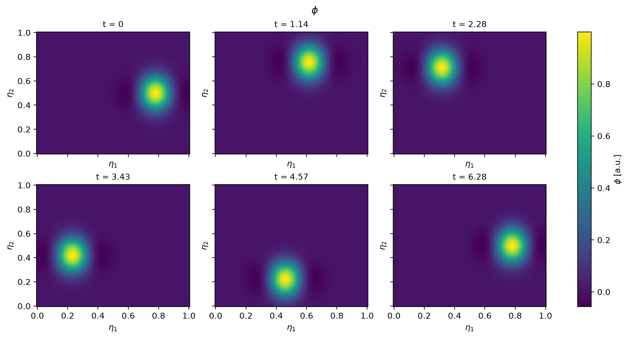
A wave packet on the unit square: a synthetic potential on a 2-D grid, drawn with array.plasma.plot the way a simulation’s output is.
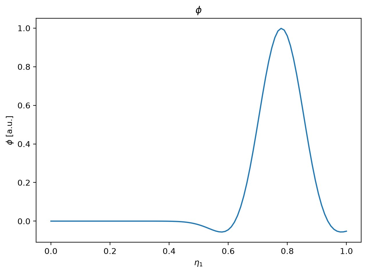
The labeled xarray.DataArray carries its coordinates, label and units, so slice, panels and
lineout need nothing more than the names of the dimensions to draw. Dimensions that a plot does not
draw are selected by keyword: an integer is a position (t=-1 the last time), a float the nearest
coordinate value.
Source code
Section titled “Source code”import matplotlib.pyplot as pltimport numpy as npimport xarray as xr
import plasma_plots # noqa: F401 (registers .plasma on DataArray)
t = np.linspace(0.0, 2 * np.pi, 12)eta1 = np.linspace(0.0, 1.0, 96)eta2 = np.linspace(0.0, 1.0, 96)E1, E2 = np.meshgrid(eta1, eta2, indexing="ij")
values = np.empty((t.size, eta1.size, eta2.size))for i, ti in enumerate(t): c1, c2 = 0.5 + 0.28 * np.cos(ti), 0.5 + 0.28 * np.sin(ti) values[i] = np.exp(-((E1 - c1) ** 2 + (E2 - c2) ** 2) / (2 * 0.1**2)) * np.cos( 10.0 * (E1 - c1) )
phi = xr.DataArray( values, dims=("t", "eta1", "eta2"), coords={"t": t, "eta1": eta1, "eta2": eta2}, name="phi", attrs={"label": r"$\phi$", "units": "a.u."},)
phi.plasma.plot.panels(x="eta1", y="eta2", nrows=2, ncols=3)phi.plasma.plot.lineout(x="eta1", t=-1, eta2=0.5)plt.show()