GVEC equilibria
GVEC computes 3-D MHD equilibria and evaluates them into
xarray Datasets: state.evaluate(...) on its logical grid, state.evaluate_sfl(...) on a
Boozer or PEST grid. plasma-plots reads those Datasets directly, whether fresh from a State or
saved with to_netcdf and opened again, so plotting a saved equilibrium does not need GVEC at all.
For DESC’s equilibria, see DESC equilibria.
import gvecimport plasma_plots
state = gvec.find_state("path/to/run")  # or run.state after gvec.run(params)ev = plasma_plots.from_gvec(    state.evaluate(        "mod_B",        "pos",        "X1",        "X2",        "Jac",        "iota",        "p",        "theta_P",        "N_FP",        rho=17,        theta=64,        zeta=40,    ))
Every figure on this page comes from real GVEC runs, made while the docs are built
(scripts/generate_gvec_figures.py, at the end of the page): the three-period stellarator and
the tokamak of GVEC’s own tutorials, and W7-X from GVEC’s examples.
Reading GVEC’s Datasets
Section titled “Reading GVEC’s Datasets”.plasma on a GVEC Dataset or one of its variables reads GVEC’s layout by itself:
ev.mod_B.plasma.plot.slice(x="zeta", y="theta", rho=1.0) works on the raw output.
plasma_plots.from_gvec(ev) does the same once for the whole Dataset, and attaches the geometry
(pos) to every variable. A single variable like ev.mod_B doesn’t carry pos, so call it
before plotting in physical space. What changes:
| GVEC | plasma-plots |
|---|---|
dimensions rad, pol, tor |
rho, theta/theta_B/theta_P, zeta/zeta_B: select with rho=0.5, draw with x="zeta" |
pos over xyz |
the coordinates X, Y, Z of every variable: coords="physical", 3-D views, gradients |
X1, X2, theta_P, a Boozer grid’s theta, zeta |
coordinates of every variable: plane="X1X2", coordinate lines |
vectors along xyz |
along component (Cartesian), as for Struphy’s vectors |
symbol attributes |
label ($\iota$), for axes and color bars |
N_FP |
the nfp attribute; the angles get a period (2π, 2π/nfp) |
rad_weight, pol_weight, tor_weight |
rho_weight, theta_weight, zeta_weight, used by integrals |
The angles stay in radians. Every other plot and diagnostic of plasma-plots then works on GVEC
data as on Struphy’s, e.g. ev.mod_B.plasma.analysis.gradient().
Poloidal planes
Section titled “Poloidal planes”ev.mod_B.plasma.plot.panels( sweep="zeta", coords="physical", plane="RZ", nrows=1, ncols=3, overlays={"coordinate_lines": {"rho": 4, "theta_P": 8}},)The field in the (R, Z) plane at three toroidal angles of one field period of the stellarator,
with four flux surfaces and eight lines of constant PEST angle θ* on top. coordinate_lines
draws lines of constant value of either drawn dimension ({"rho": 4, "theta": 8} for GVEC’s own
angle), or contour lines of another coordinate over them, here theta_P (evaluate it with the
rest). An angle gets its lines spread over its period and none twice at its seam. A number gives
that many lines, a list the values themselves ({"rho": [0.5, 1.0]}). slice(..., zeta=0.0)
draws one plane. plane="X1X2" draws GVEC’s reference coordinates instead: the same as "RZ"
for the cylindrical map, the plane of the curved frame for the others.
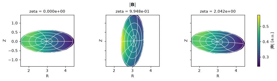
The data behind one of these planes: ev.mod_B.plasma.data.slice(coords="physical", plane="RZ", zeta=0.0) returns the selected field, with its X, Y, Z (see Selecting data).
The same plot with Plotly
One plane, with backend="plotly" (see Interactive plots with Plotly).
ev.mod_B.plasma.plot.slice( coords="physical", plane="RZ", zeta=0.0, overlays={"coordinate_lines": {"rho": 4, "theta_P": 8}}, backend="plotly",)Loading interactive chart…
The same for W7-X, from the bean-shaped plane at zeta = 0 over half a field period to the
triangular one:
planes = plasma_plots.from_gvec( w7x.evaluate( "mod_B", "pos", "X1", "X2", "theta_P", "N_FP", rho=13, theta=96, zeta=np.linspace(0, np.pi / w7x.nfp, 3), ))planes.mod_B.plasma.plot.panels( sweep="zeta", coords="physical", plane="RZ", nrows=1, ncols=3, overlays={"coordinate_lines": {"rho": 4, "theta_P": 12}},)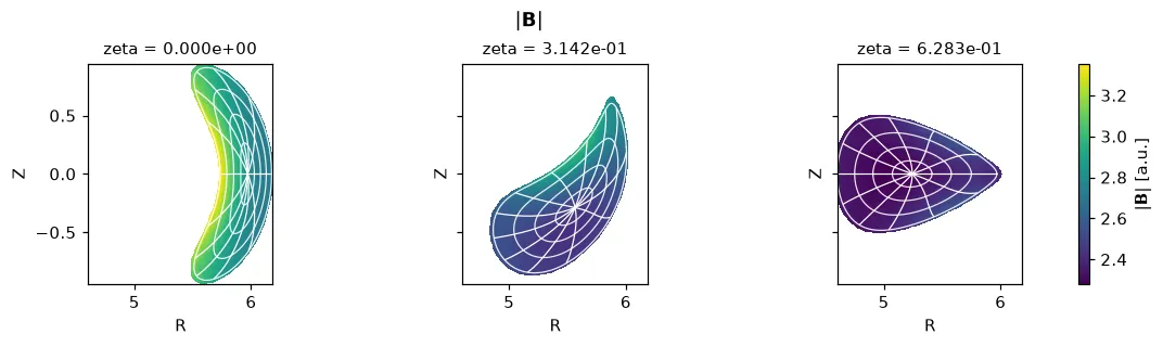
On a flux surface
Section titled “On a flux surface”boozer = plasma_plots.from_gvec( state.evaluate_sfl( "mod_B", "pos", "N_FP", rho=np.linspace(0.1, 1.0, 10), theta=64, zeta=40, sfl="boozer", ))with plasma_plots.figure(1, 2) as fig: ev.mod_B.plasma.plot.slice( x="zeta", y="theta", rho=0.5, levels=12, ax=fig[0] ) boozer.mod_B.plasma.plot.slice( x="zeta_B", y="theta_B", rho=0.5, levels=12, ax=fig[1] )A surface is a logical slice at one rho: here |B| on the surface rho = 0.5, over GVEC’s
logical angles (left) and over the Boozer angles of an evaluate_sfl grid (right); PEST’s is
x="zeta", y="theta_P". levels=12 adds contour lines.
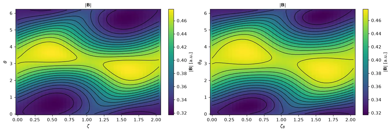
The data behind these plots: boozer.mod_B.plasma.data.slice(x="zeta_B", y="theta_B", rho=0.5) and the same of ev.mod_B.
The same plot with Plotly
boozer.mod_B.plasma.plot.slice( x="zeta_B", y="theta_B", rho=0.5, levels=12, backend="plotly")Loading interactive chart…
A Boozer grid carries GVEC’s logical angles as coordinates, so coordinate_lines draws where they
are constant, the way GVEC’s own Boozer tutorial shows the transform:
boozer.mod_B.plasma.plot.slice( x="zeta_B", y="theta_B", rho=0.5, overlays={"coordinate_lines": {"theta": 12, "zeta": 8}},)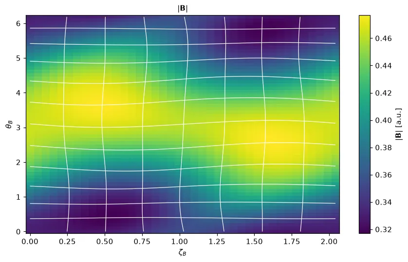
For axes in units of 2π, as GVEC labels them, rescale the angles first:
boozer.mod_B.plasma.analysis.map_coordinate("theta_B", 1 / (2 * np.pi), label=r"$\theta_B / 2\pi$"),
and the same for zeta_B. The rescaled angle is for display: it no longer has GVEC’s period.
Fourier modes
Section titled “Fourier modes”boozer.mod_B.plasma.plot.mode_map(rho=0.5, m_range=(-4, 4), n_range=(-9, 9))The amplitudes of |B| on the surface rho = 0.5 over poloidal m and toroidal n. On GVEC’s
angles the transform takes their periods from the Dataset, so n is the full-torus mode number,
a multiple of nfp (here 3). boozer.mod_B.plasma.analysis.mode_spectrum() returns the complex
amplitudes over (rho, m, n), e.g. for measures of quasi-symmetry. See
Spectral analysis for the other mode tools.
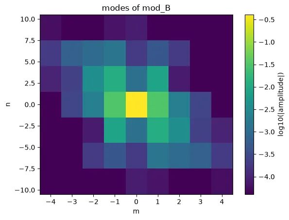
The data behind this plot: abs(boozer.mod_B.plasma.analysis.mode_spectrum()).sel(rho=0.5).
The strongest harmonics over the radius, on the ten Boozer surfaces:
boozer.mod_B.plasma.plot.mode_profiles(top=5)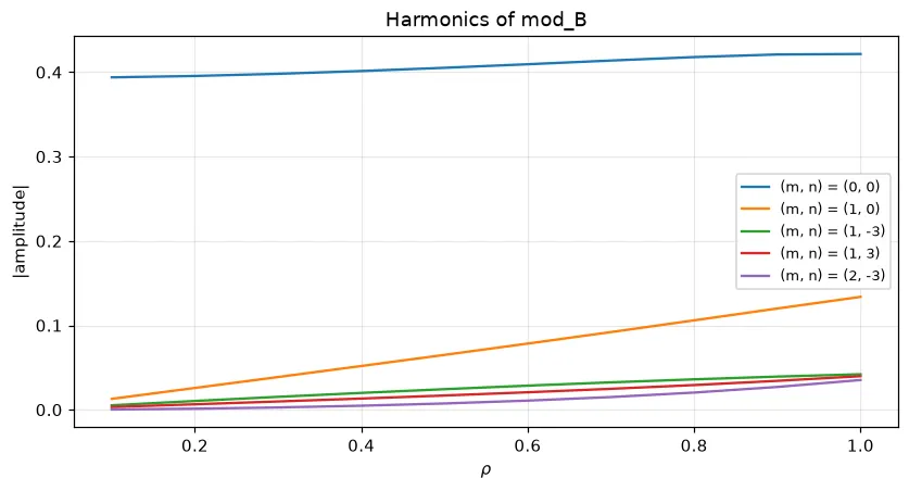
Boozer spectrum and quasi-symmetry
Section titled “Boozer spectrum and quasi-symmetry”B_mn = boozer.mod_B.plasma.analysis.boozer_spectrum(top=8)f_qs = boozer.mod_B.plasma.analysis.quasisymmetry_error(helicity="QA")boozer.mod_B.plasma.plot.boozer_spectrum(top=8, helicity="QA")In Boozer angles the spectrum of |B| is what the guiding-center drifts see. boozer_spectrum
gives the real harmonics B_mn(ρ) (Σ B_mn cos(m θ_B + n ζ_B), with n the full-torus mode
number; the usual stellarator convention cos(m θ_B − n ζ_B) has the opposite sign of n), the
strongest first. A field is quasi-symmetric with helicity (M, N) when |B| depends on the
angles only through M θ_B − N ζ_B; quasisymmetry_error is the symmetry-breaking content
relative to the mean field, f_QS(ρ) = √(Σ_breaking B_mn²) / B_00, for "QA"
(quasi-axisymmetry, N = 0), "QP" (M = 0), "QH" ((1, nfp), either handedness) or a
pair (M, N). The plot draws the harmonics over the radius, symmetry-breaking ones dashed, and
the error below. Both need a Boozer grid (evaluate_sfl(..., sfl="boozer")); angles="any"
takes the harmonics in whatever angles the field has.
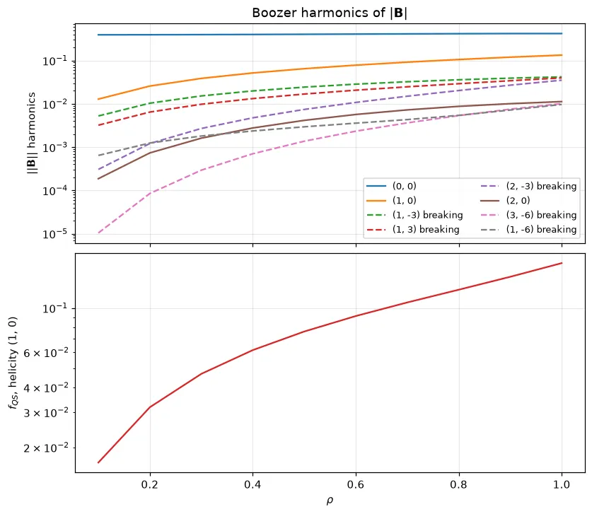
Profiles
Section titled “Profiles”with plasma_plots.figure(2, 2) as fig: ev.iota.plasma.plot.lineout(rationals=4, ax=fig[0]) ev.p.plasma.plot.lineout(ax=fig[1]) ev.plasma.analysis.surface_average("mod_B").plasma.plot.lineout(ax=fig[2]) # on the magnetic axis ev.mod_B.plasma.plot.lineout(x="zeta", rho=0, theta=0, ax=fig[3])rationals=4 marks the four lowest-order rational values n/m of ι that the profile reaches,
with n a multiple of nfp (the resonances of a device with nfp field periods), and the radius
of each crossing. ev.iota.plasma.analysis.rational_surfaces(count=4) returns them as an array
over surface, with the coordinates n, m and value.
surface_average is ⟨f⟩ = ∫ f √g dθ dζ / ∫ √g dθ dζ over both angles. On a Dataset,
ev.plasma.analysis.surface_average("mod_B") takes GVEC’s Jacobian Jac (evaluate it with the
rest); on one variable, pass it: ev.mod_B.plasma.analysis.surface_average(jacobian=ev.Jac).
Without one, √g comes from the numerical Jacobian of X, Y, Z, which is accurate to a
fraction of a percent on a fine grid. On the magnetic axis, where √g vanishes, it is the plain
mean over the angles.
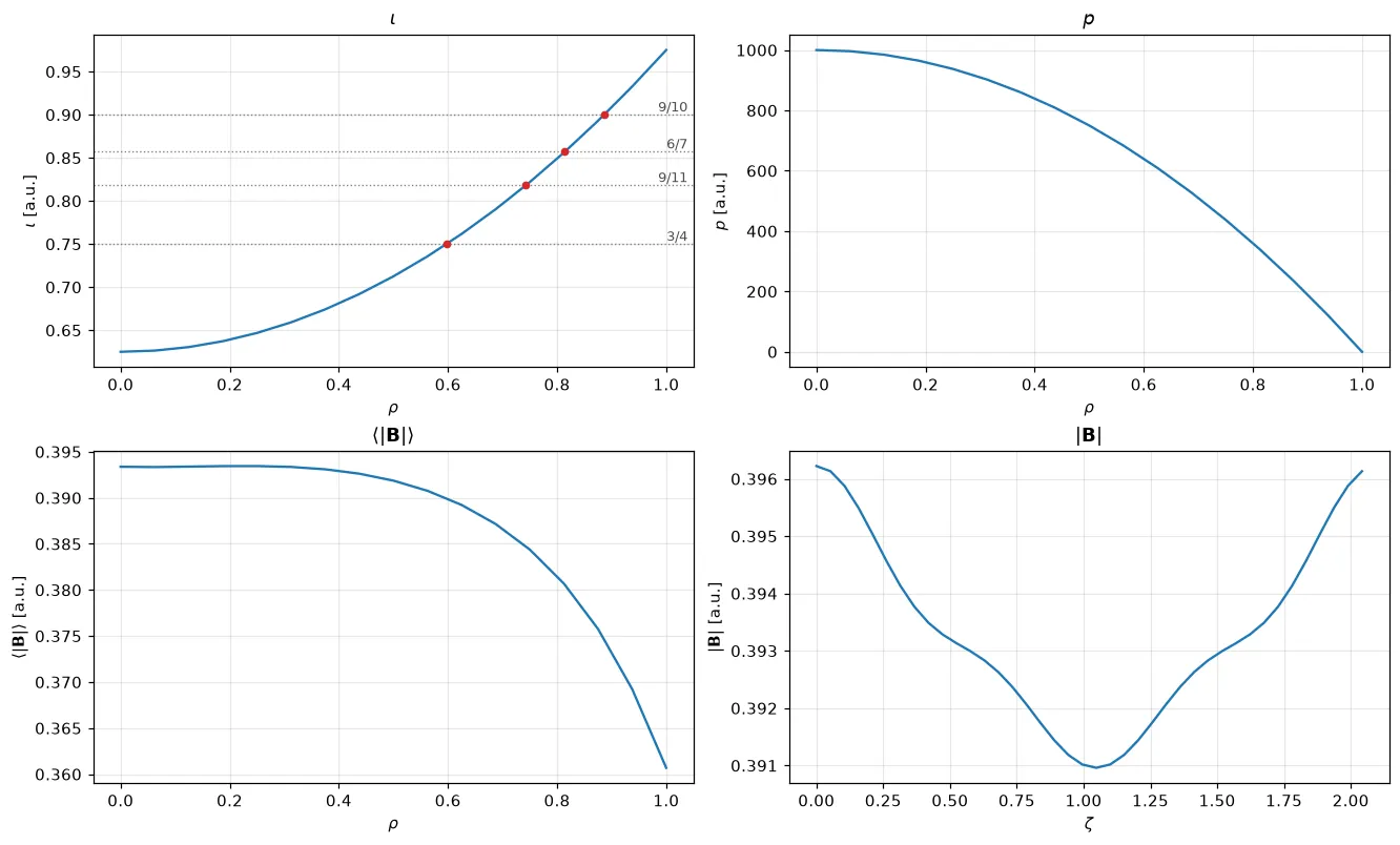
The data behind these plots: ev.iota.plasma.data.lineout(), the surface_average array itself, and so on.
The same plot with Plotly
ev.iota.plasma.plot.lineout(rationals=4, backend="plotly")Loading interactive chart…
For a tokamak, the safety factor q = 1/ι works the same way; here with the tokamak’s poloidal
plane next to it:
tok = plasma_plots.from_gvec( tokamak.evaluate( "mod_B", "pos", "X1", "X2", "iota", "theta_P", "N_FP", rho=17, theta=64, zeta=[0.0], ))q = (1 / tok.iota).rename("q")q.attrs = {"label": "$q$", "nfp": 1}with plasma_plots.figure(1, 2) as fig: tok.mod_B.plasma.plot.slice( coords="physical", plane="RZ", zeta=0.0, overlays={"coordinate_lines": {"rho": 5, "theta_P": 12}}, ax=fig[0], ) q.plasma.plot.lineout(rationals=4, ax=fig[1])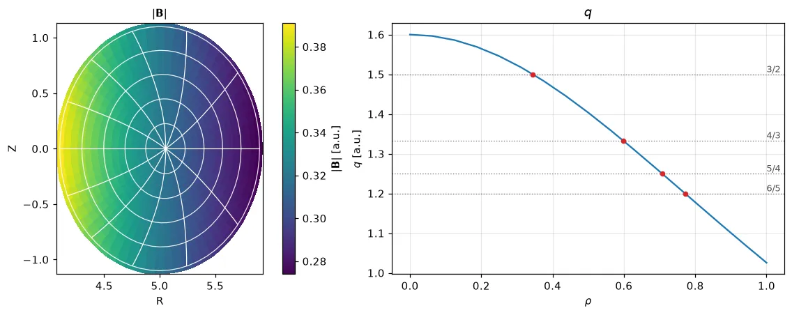
Integrals
Section titled “Integrals”import xarray as xrfrom plasma_plots.analysis import volume_integral
gauss = plasma_plots.from_gvec( state.evaluate( "mod_B", "Jac", "pos", "N_FP", rho="int", theta="int", zeta="int" ))volume = ( volume_integral(xr.ones_like(gauss.Jac), jacobian=gauss.Jac) * gauss.nfp)volume_integral integrates over the sampled grid, which covers one field period, so multiply by
nfp for the whole device. On GVEC’s integration points ("int") it uses GVEC’s Gauss weights
(GVEC’s toroidal weight counts all field periods; from_gvec rescales it to one). On a uniform
grid the angles get the rectangle rule, which is exact for their Fourier modes, and the radius
the trapezoidal rule. jacobian= takes GVEC’s Jac; without it, √g comes from the geometry.
For the stellarator, against GVEC’s own volume (state.evaluate("V", rho=[1.0])):
plasma volume, GVEC's own V                      49.7428061815
volume_integral(1, jacobian=Jac) * nfp, Gauss    49.7428061815
volume_integral(1) * nfp, sqrt(g) from X, Y, Z   49.6914247226
<|B|> at rho = 0.5                               0.3918639104
In 3-D
Section titled “In 3-D”With PyVista (see 3-D views), on a grid over the whole torus
(every field period) with the field B evaluated too. cuts take rho, theta and zeta like
Struphy’s eta1, eta2, eta3.
torus = plasma_plots.from_gvec( state.evaluate( "mod_B", "B", "pos", "N_FP", rho=9, theta=48, zeta=np.linspace(0, 2 * np.pi, 32 * state.nfp, endpoint=False), ))torus.mod_B.plasma.plot.slices_3d(cuts={"rho": [1.0]}).show()|B| on the last flux surface:
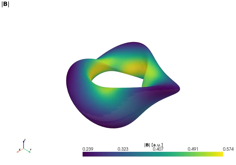
Drag to rotate, scroll to zoom, shift-drag to pan.Open in a new tab
An inner surface and three poloidal cuts, inside the translucent outer surface:
torus.mod_B.plasma.plot.slices_3d( cuts={"rho": [0.5], "zeta": [0.0, np.pi / 2, np.pi]}).show()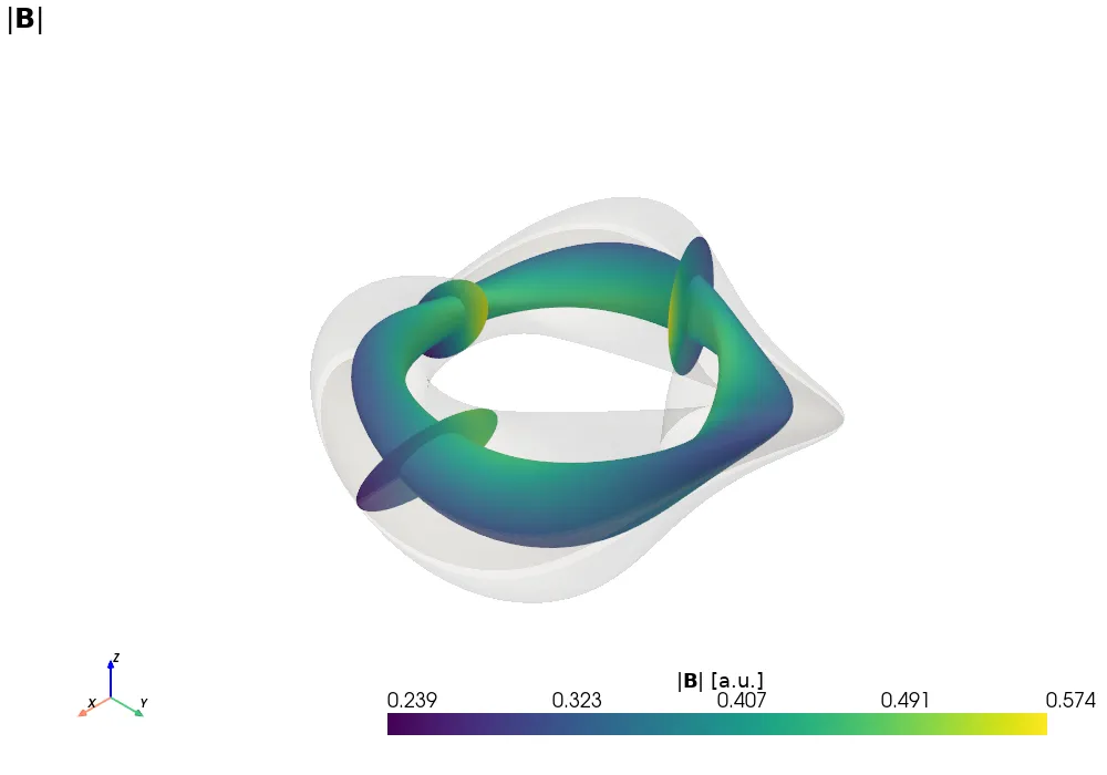
Drag to rotate, scroll to zoom, shift-drag to pan.Open in a new tab
Magnetic field lines, traced through GVEC’s B from a small sphere of seeds next to the axis:
axis = torus.isel(rho=0, theta=0, zeta=0)torus.B.plasma.plot.streamlines( n_points=40, source_center=(float(axis.X) + 0.35, float(axis.Y), float(axis.Z)), source_radius=0.25, tube_radius=0.015,).show()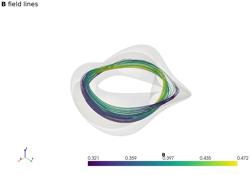
Drag to rotate, scroll to zoom, shift-drag to pan.Open in a new tab
And W7-X’s last flux surface, all five field periods:
surface = plasma_plots.from_gvec( w7x.evaluate( "mod_B", "pos", "N_FP", rho=[1.0], theta=64, zeta=np.linspace(0, 2 * np.pi, 48 * w7x.nfp, endpoint=False), ))surface.mod_B.plasma.plot.slices_3d().show()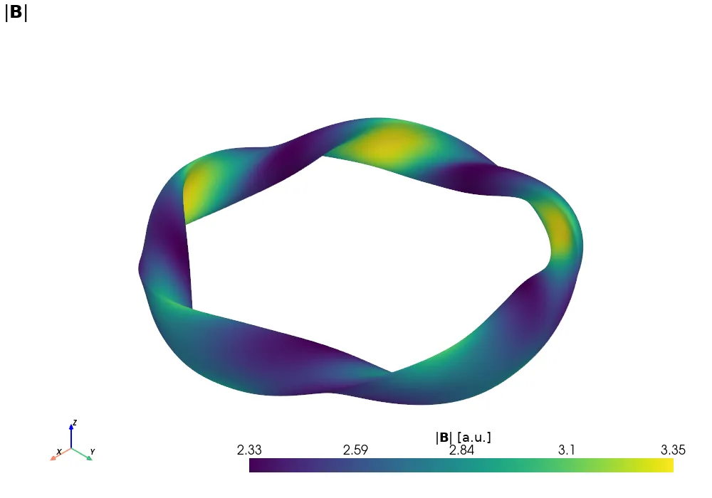
Drag to rotate, scroll to zoom, shift-drag to pan.Open in a new tab
The script behind this page
Section titled “The script behind this page”It runs the three equilibria (W7-X takes about a minute) and writes every figure above.
scripts/generate_gvec_figures.py, unedited
"""Generate the figures of the "GVEC equilibria" guide
(docs/src/assets/figures/gvec_*) from real GVEC equilibria.

Like ``generate_real_example_figures.py`` for Struphy, this runs the actual
code: GVEC's own tutorial equilibria (a three-period stellarator and a tokamak,
from GVEC's docs), and W7-X from GVEC's examples, evaluated with
``state.evaluate`` / ``state.evaluate_sfl`` and plotted with plasma-plots. It
needs ``pip install gvec``, which builds GVEC's Fortran core (gfortran, a
LAPACK); the interactive 3-D scenes need PyVista and trame-pyvista, the Plotly
charts plotly (see .github/workflows/docs.yml).

Run from the repo root: python scripts/generate_gvec_figures.py (or: make
figures). W7-X takes a few minutes; set PLASMA_PLOTS_SKIP_W7X=1 to leave it
out.
"""

from __future__ import annotations

import os

os.environ.setdefault("OMP_NUM_THREADS", "2")  # before importing gvec

import sys
import tempfile
import time
from pathlib import Path

import matplotlib

matplotlib.use("Agg")

import gvec
import matplotlib.pyplot as plt
import numpy as np
import xarray as xr

sys.path.insert(0, str(Path(__file__).resolve().parents[1] / "src"))
import plasma_plots
from plasma_plots.analysis import volume_integral

ROOT = Path(__file__).resolve().parents[1]
DOCS = ROOT / "docs"
OUT = DOCS / "src" / "assets" / "figures"
NUMBERS = DOCS / "src" / "assets" / "gvec" / "numbers.txt"
PLOTLY_OUT = DOCS / "public" / "plotly"
PYVISTA_OUT = DOCS / "public" / "pyvista"
for folder in (OUT, NUMBERS.parent, PLOTLY_OUT, PYVISTA_OUT):
    folder.mkdir(parents=True, exist_ok=True)
WORK = Path(tempfile.mkdtemp(prefix="gvec-runs-"))


def save(result, filename):
    result.save(OUT / filename, close=True)
    print(f"wrote {OUT / filename}")


def save_plotly(result, filename):
    print(f"wrote {result.save(PLOTLY_OUT / f'{filename}.json')}")


def equilibrium(parameters, name):
    """Run GVEC and return its final State."""
    start = time.time()
    run = gvec.run(parameters, runpath=WORK / name, quiet=True)
    print(f"GVEC {name}: {time.time() - start:.1f} s")
    return run.state


# =============================================================================
# The equilibria: GVEC's tutorial stellarator (docs/tutorials 051_plotting,
# three field periods, a rotating ellipse), its tutorial tokamak (010_tokamak,
# elliptic), and W7-X (examples/).
# =============================================================================
STELLARATOR = {
    "ProjectName": "stellarator",
    "which_hmap": 1,
    "PhiEdge": 1.0,
    "iota": {"type": "polynomial", "coefs": [0.625, 0.35]},
    "pres": {"type": "polynomial", "coefs": [1.0, -1.0], "scale": 1000.0},
    "nfp": 3,
    "X1_b_cos": {(0, 0): 3.0, (1, 0): 1.0, (1, 1): 0.4},
    "X2_b_sin": {(1, 0): 1.0, (1, 1): -0.4, (0, 1): -0.25},
    "init_average_axis": True,
    "sgrid_nElems": 2,
    "X1_mn_max": [3, 3],
    "X2_mn_max": [3, 3],
    "LA_mn_max": [3, 3],
    "X1X2_deg": 5,
    "LA_deg": 5,
    "totalIter": 1000,
    "minimize_tol": 1.0e-6,
}
TOKAMAK = {
    "ProjectName": "tokamak",
    "which_hmap": 1,
    "PhiEdge": 1.0,
    "iota": {"type": "polynomial", "coefs": [0.625, 0.35]},
    "pres": {
        "type": "interpolation",
        "rho2": [0.0, 0.25, 0.5, 0.75, 1.0],
        "vals": [1.0, 0.75, 0.5, 0.25, 0.0],
        "scale": 1000.0,
    },
    "nfp": 1,
    "X1_b_cos": {(0, 0): 5.0, (1, 0): 0.9},
    "X2_b_sin": {(1, 0): 1.1},
    "X1_a_cos": {(0, 0): 5.0},
    "X1_mn_max": [3, 0],
    "X2_mn_max": [3, 0],
    "LA_mn_max": [3, 0],
    "sgrid_nElems": 2,
    "X1X2_deg": 5,
    "LA_deg": 5,
    "totalIter": 10000,
    "minimize_tol": 1e-6,
}

stellarator = equilibrium(STELLARATOR, "stellarator")
nfp = stellarator.nfp
# one field period, on GVEC's logical angles; the geometry (pos) and the grid
# (X1, X2, theta_P) go on every variable with from_gvec
ev = plasma_plots.from_gvec(
    stellarator.evaluate(
        "mod_B",
        "pos",
        "X1",
        "X2",
        "Jac",
        "iota",
        "p",
        "theta_P",
        "N_FP",
        rho=17,
        theta=64,
        zeta=40,
    )
)
# the same field period on a Boozer grid, on ten flux surfaces
boozer = plasma_plots.from_gvec(
    stellarator.evaluate_sfl(
        "mod_B",
        "pos",
        "N_FP",
        rho=np.linspace(0.1, 1.0, 10),
        theta=64,
        zeta=40,
        sfl="boozer",
    )
)

# =============================================================================
# Poloidal planes
# =============================================================================
lines = {"coordinate_lines": {"rho": 4, "theta_P": 8}}
save(
    ev.mod_B.plasma.plot.panels(
        sweep="zeta",
        coords="physical",
        plane="RZ",
        nrows=1,
        ncols=3,
        overlays=lines,
    ),
    "gvec_poloidal_planes.png",
)

tokamak = equilibrium(TOKAMAK, "tokamak")
tok = plasma_plots.from_gvec(
    tokamak.evaluate(
        "mod_B",
        "pos",
        "X1",
        "X2",
        "iota",
        "theta_P",
        "N_FP",
        rho=17,
        theta=64,
        zeta=[0.0],
    )
)
q = (1 / tok.iota).rename("q")
q.attrs = {"label": "$q$", "nfp": 1}
with plasma_plots.figure(1, 2) as fig:
    tok.mod_B.plasma.plot.slice(
        coords="physical",
        plane="RZ",
        zeta=0.0,
        overlays={"coordinate_lines": {"rho": 5, "theta_P": 12}},
        ax=fig[0],
    )
    q.plasma.plot.lineout(rationals=4, ax=fig[1])
save(fig, "gvec_tokamak.png")

# =============================================================================
# On a flux surface: GVEC's own angles and Boozer's, and the logical angles
# over the Boozer grid
# =============================================================================
with plasma_plots.figure(1, 2) as fig:
    ev.mod_B.plasma.plot.slice(
        x="zeta", y="theta", rho=0.5, levels=12, ax=fig[0]
    )
    boozer.mod_B.plasma.plot.slice(
        x="zeta_B", y="theta_B", rho=0.5, levels=12, ax=fig[1]
    )
save(fig, "gvec_surfaces.png")
save(
    boozer.mod_B.plasma.plot.slice(
        x="zeta_B",
        y="theta_B",
        rho=0.5,
        overlays={"coordinate_lines": {"theta": 12, "zeta": 8}},
    ),
    "gvec_boozer_grid.png",
)

# =============================================================================
# Fourier modes of |B| on the Boozer grid
# =============================================================================
save(
    boozer.mod_B.plasma.plot.mode_map(
        rho=0.5, m_range=(-4, 4), n_range=(-9, 9)
    ),
    "gvec_mode_map.png",
)
save(boozer.mod_B.plasma.plot.mode_profiles(top=5), "gvec_mode_profiles.png")
save(
    boozer.mod_B.plasma.plot.boozer_spectrum(top=8, helicity="QA"),
    "gvec_boozer_spectrum.png",
)

# =============================================================================
# Profiles: the rotational transform with its rational surfaces, the pressure,
# <|B|>, |B| on axis
# =============================================================================
with plasma_plots.figure(2, 2) as fig:
    ev.iota.plasma.plot.lineout(rationals=4, ax=fig[0])
    ev.p.plasma.plot.lineout(ax=fig[1])
    ev.plasma.analysis.surface_average("mod_B").plasma.plot.lineout(ax=fig[2])
    ev.mod_B.plasma.plot.lineout(x="zeta", rho=0, theta=0, ax=fig[3])
save(fig, "gvec_profiles.png")

# =============================================================================
# Numbers: the volume from GVEC's Jacobian on its integration points, against
# GVEC's own
# =============================================================================
gauss = plasma_plots.from_gvec(
    stellarator.evaluate(
        "mod_B", "Jac", "pos", "N_FP", rho="int", theta="int", zeta="int"
    )
)
volume = (
    float(volume_integral(xr.ones_like(gauss.Jac), jacobian=gauss.Jac))
    * gauss.nfp
)
numerical = float(volume_integral(xr.ones_like(ev.mod_B))) * ev.nfp
gvec_volume = float(stellarator.evaluate("V", rho=[1.0]).V)
average = ev.plasma.analysis.surface_average("mod_B")
rows = [
    ("plasma volume, GVEC's own V", gvec_volume),
    ("volume_integral(1, jacobian=Jac) * nfp, Gauss", volume),
    ("volume_integral(1) * nfp, sqrt(g) from X, Y, Z", numerical),  # 17x64x40
    ("<|B|> at rho = 0.5", float(average.sel(rho=0.5))),
]
NUMBERS.write_text(
    "".join(f"{label:<48} {value:.10f}\n" for label, value in rows)
)
print(NUMBERS.read_text())

# =============================================================================
# Interactive 3-D: the whole stellarator (every field period), a cutaway and
# field lines
# =============================================================================
try:
    import pyvista as pv

    pv.OFF_SCREEN = True

    def shot(plotter, filename, *, zoom=1.0, camera="iso"):
        """A PNG, and an interactive HTML scene for <PyVistaScene>."""
        plotter.camera_position = camera
        plotter.reset_camera()
        plotter.camera.zoom(zoom)
        plotter.screenshot(str(OUT / filename), window_size=[1000, 700])
        print(f"wrote {OUT / filename}")
        html = PYVISTA_OUT / filename.replace(".png", ".html")
        # vtk.js would show them 0-255
        for title in list(plotter.scalar_bars.keys()):
            plotter.remove_scalar_bar(title)
        try:
            plotter.trame.export_html(str(html))
            print(f"wrote {html}")
        except Exception as exc:  # needs trame-pyvista
            print(
                f"skipped {html.name} (interactive export unavailable): {exc}"
            )
        plotter.close()

    torus = plasma_plots.from_gvec(
        stellarator.evaluate(
            "mod_B",
            "B",
            "pos",
            "N_FP",
            rho=9,
            theta=48,
            zeta=np.linspace(0, 2 * np.pi, 32 * nfp, endpoint=False),
        )
    )
    shot(
        torus.mod_B.plasma.plot.slices_3d(cuts={"rho": [1.0]}),
        "gvec_3d_surface.png",
    )
    shot(
        torus.mod_B.plasma.plot.slices_3d(
            cuts={"rho": [0.5], "zeta": [0.0, np.pi / 2, np.pi]}
        ),
        "gvec_3d_cutaway.png",
    )
    axis = torus.isel(rho=0, theta=0, zeta=0)
    shot(
        torus.B.plasma.plot.streamlines(
            n_points=40,
            source_center=(float(axis.X) + 0.35, float(axis.Y), float(axis.Z)),
            source_radius=0.25,
            tube_radius=0.015,
        ),
        "gvec_3d_fieldlines.png",
    )
except ImportError as exc:  # pragma: no cover - optional
    print(f"skipped the 3-D views (pyvista unavailable): {exc}")

# =============================================================================
# W7-X (GVEC's examples/parameter-w7x.toml, in scripts/data; five field
# periods): planes and its last surface
# =============================================================================
if not os.environ.get("PLASMA_PLOTS_SKIP_W7X"):
    from gvec.util import read_parameters

    # a copy of the file: the sdist does not install GVEC's examples
    w7x = equilibrium(
        read_parameters(ROOT / "scripts" / "data" / "gvec-parameter-w7x.toml"),
        "w7x",
    )
    planes = plasma_plots.from_gvec(
        w7x.evaluate(
            "mod_B",
            "pos",
            "X1",
            "X2",
            "theta_P",
            "N_FP",
            rho=13,
            theta=96,
            zeta=np.linspace(0, np.pi / w7x.nfp, 3),
        )
    )
    save(
        planes.mod_B.plasma.plot.panels(
            sweep="zeta",
            coords="physical",
            plane="RZ",
            nrows=1,
            ncols=3,
            overlays={"coordinate_lines": {"rho": 4, "theta_P": 12}},
        ),
        "gvec_w7x_planes.png",
    )
    try:
        import pyvista as pv  # noqa: F811

        surface = plasma_plots.from_gvec(
            w7x.evaluate(
                "mod_B",
                "pos",
                "N_FP",
                rho=[1.0],
                theta=64,
                zeta=np.linspace(0, 2 * np.pi, 48 * w7x.nfp, endpoint=False),
            )
        )
        shot(
            surface.mod_B.plasma.plot.slices_3d(), "gvec_3d_w7x.png", zoom=1.3
        )
    except ImportError as exc:  # pragma: no cover - optional
        print(f"skipped the W7-X 3-D view (pyvista unavailable): {exc}")

# =============================================================================
# The same plots with Plotly (the folds in the guide)
# =============================================================================
try:
    import plotly  # noqa: F401

    save_plotly(
        ev.mod_B.plasma.plot.slice(
            coords="physical",
            plane="RZ",
            zeta=0.0,
            overlays=lines,
            backend="plotly",
        ),
        "plotly_gvec_poloidal_plane",
    )
    save_plotly(
        boozer.mod_B.plasma.plot.slice(
            x="zeta_B", y="theta_B", rho=0.5, levels=12, backend="plotly"
        ),
        "plotly_gvec_boozer_surface",
    )
    save_plotly(
        ev.iota.plasma.plot.lineout(rationals=4, backend="plotly"),
        "plotly_gvec_iota",
    )
except ImportError as exc:  # pragma: no cover - optional
    print(f"skipped the Plotly figures (plotly unavailable): {exc}")

plt.close("all")
print("done")