Space-charge-limited flow
Child–Langmuir and Langmuir–Blodgett space-charge-limited flow: how curvature changes the space-charge-limited current of a diode, against the planar Child–Langmuir law.
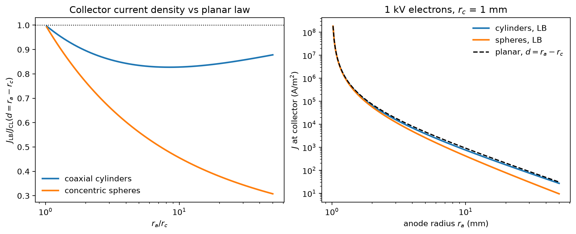
The planar law is exact for parallel plates. For coaxial cylinders and concentric spheres the Langmuir–Blodgett series gives the current density at the collector. With the emitter inside, the collector area is larger and the density at the collector is lower than the planar value, by a factor that grows with the radius ratio . The planar limit is recovered as .
Source code
Section titled “Source code”import matplotlib.pyplot as pltimport numpy as np
from plasma_plots.theory import sheaths
voltage = 1e3 # V, electronsr_c = 1e-3 # mratio = np.geomspace(1.02, 50, 200)r_a = ratio * r_c
planar = sheaths.child_langmuir(voltage, r_a - r_c)cyl = sheaths.langmuir_blodgett(voltage, r_a, r_c, geometry="cylindrical")sph = sheaths.langmuir_blodgett(voltage, r_a, r_c, geometry="spherical")
fig, (ax_r, ax_i) = plt.subplots(1, 2, figsize=(10, 4), layout="constrained")ax_r.semilogx(ratio, cyl / planar, lw=2, label="coaxial cylinders")ax_r.semilogx(ratio, sph / planar, lw=2, label="concentric spheres")ax_r.axhline(1, color="k", ls=":", lw=1)ax_r.set( xlabel=r"$r_a / r_c$", ylabel=r"$J_\mathrm{LB} / J_\mathrm{CL}(d = r_a - r_c)$", title="Collector current density vs planar law",)ax_r.legend(frameon=False)
ax_i.loglog(r_a * 1e3, cyl, lw=2, label="cylinders, LB")ax_i.loglog(r_a * 1e3, sph, lw=2, label="spheres, LB")ax_i.loglog(r_a * 1e3, planar, "k--", lw=1.5, label="planar, $d = r_a - r_c$")ax_i.set( xlabel=r"anode radius $r_a$ (mm)", ylabel=r"$J$ at collector (A/m$^2$)", title=rf"1 kV electrons, $r_c$ = {r_c * 1e3:.0f} mm",)ax_i.legend(frameon=False)
j_ratio = sheaths.langmuir_blodgett(voltage, 5e-3, r_c) / sheaths.child_langmuir( voltage, 4e-3)print(f"r_a/r_c = 5, cylinders: J_LB/J_CL = {j_ratio:.4f}")plt.show()Printed output
r_a/r_c = 5, cylinders: J_LB/J_CL = 0.8348