Recipes
Some diagnostics in the Struphy examples are a line or two of xarray on Struphy’s labeled output, so plasma-plots has no function for them. Here they are as recipes. Other diagnostics are specific to one setup, such as the Lagrangian cell areas of the Beltrami example, which need markers loaded on a lattice; those stay with their examples.
Front position and center of mass
Section titled “Front position and center of mass”For a dam break, from the orbits of the fluid markers:
orbits = out.evaluate("euler_fluid")front = orbits.x.max("marker") # the fluid's leading edge# the center of mass falls as the column collapsesheight = orbits.y.mean("marker")front.plasma.plot.timeseries(height, logy=False)arrival = float(front.t[int((front >= 0.95).argmax())])Error against an analytic solution
Section titled “Error against an analytic solution”For a field, use error(),
with the exact solution as a function of x, y, z, t:
u.plasma.analysis.error( lambda x, y, z, t: np.sin(x - t), relative=True).plasma.plot.timeseries()For markers, with the exact velocity v1_exact, v2_exact evaluated at the
marker positions (e.g. of a Beltrami flow), the relative RMS error over time:
error = np.sqrt( ((orbits.v1 - v1_exact) ** 2 + (orbits.v2 - v2_exact) ** 2).mean("marker"))error = error / np.sqrt((orbits.v1**2 + orbits.v2**2).isel(t=0).mean("marker"))error.plasma.plot.timeseries()For a conserved quantity per marker, e.g. the Hamiltonian H, the largest
relative drift is abs(H - H.isel(t=0)).max("marker") / abs(H.isel(t=0)).
For the speed of full orbits and the energy of guiding centers, use
orbit_invariants().
For a scalar time series, use .plasma.analysis.relative_error().
Frequency or period of a signal
Section titled “Frequency or period of a signal”Several examples count zero crossings or read the distance between maxima. A spectral peak is more accurate, and it does not need a clean signal:
# refined below the bin spacingpeaks = probe.plasma.analysis.spectral_peaks(n_peaks=1)period = 2 * np.pi / float(peaks.omega_refined[0])
# frequency and growth rate from a short recordfit = probe.plasma.analysis.matrix_pencil(n_modes=1)
See power spectra and frequency and growth from a short record.
From power_spectrum_2d to the dispersion plot
Section titled “From power_spectrum_2d to the dispersion plot”Older scripts call Struphy’s power_spectrum_2d on arrays loaded by hand, with
the grid spacings and the branches passed separately. On a labeled field, the
same diagram is one call, and the spectrum itself another:
e1 = out.evaluate("e_field", eta2=0.0, eta3=0.0).sel(component=0)e1.plasma.plot.dispersion( dim="eta1", branches={"Bohm-Gross": lambda k: np.sqrt(1 + 3 * k**2)})spectrum = e1.plasma.analysis.dispersion(dim="eta1") # (omega, k) powertraced = spectrum.plasma.analysis.trace_branch(lambda k: np.sqrt(1 + 3 * k**2))k and omega come from the coordinates, in the units of eta1 (or of X for
dim="X" on a slab). See tracing a branch.
Periodic wrap-around
Section titled “Periodic wrap-around”Markers in a periodic box are stored inside it, so their paths jump across the domain. Unwrap them for distances and mean-square displacements:
L = 2 * np.pix_unwrapped = orbits.x.copy( data=np.unwrap(orbits.x, period=L, axis=orbits.x.get_axis_num("t")))msd = ((x_unwrapped - x_unwrapped.isel(t=0)) ** 2).mean("marker")Tracking a peak
Section titled “Tracking a peak”The position of a wave packet’s or pulse’s maximum over time, and its speed:
envelope = abs(phi) # or a filtered envelopepeak = envelope.idxmax("eta1") # per tspeed = float(np.polyfit(peak.t, peak, 1)[0])To check it against theory, draw the expected line on a space-time map.
E×B energy of zonal flows and drift waves
Section titled “E×B energy of zonal flows and drift waves”In a 2-D drift-wave model with the potential phi, the E×B velocity is
ẑ × ∇φ, so its kinetic energy density is ½⟨|∇φ|²⟩. The zonal flow is the
part of phi averaged along y (ky = 0), and the drift waves are the rest.
Their energies add up, because the two parts are orthogonal:
grad = phi.plasma.analysis.gradient()total = 0.5 * (grad.sel(component=[0, 1]) ** 2).sum("component").mean(    ("eta1", "eta2", "eta3"))
zonal = xr.zeros_like(phi) + phi.mean("eta2")  # keeps the X, Y coordinatesgrad_zonal = zonal.plasma.analysis.gradient()zonal_energy = 0.5 * (grad_zonal.sel(component=[0, 1]) ** 2).sum(    "component").mean(("eta1", "eta2", "eta3"))
fig, ax = plt.subplots()ax.stackplot(    phi.t,    total - zonal_energy,    zonal_energy,    labels=["drift waves", "zonal flow"],)ax.legend()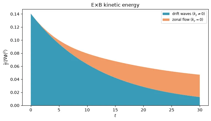
Interfaces and edges
Section titled “Interfaces and edges”For the inner and outer edge of a ring as curves, draw contour lines
(levels=[0.2], see contour lines).
For their radii at each angle as data, take the first and last radius above
the threshold:
inside = (n >= 0.2).isel(eta3=0)inner = n.eta1.where(inside).min("eta1") # per eta2 and touter = n.eta1.where(inside).max("eta1")