Field lines

Where the accessors come from

The examples on this page use output of a Struphy Output, which loads plasma-plots and its .plasma accessors. For other xarray data, run import plasma_plots first (see Getting started).

A field line follows the direction of a vector field, dx/ds = B/|B|. plasma-plots traces it in the logical coordinates of the grid, where the grid is rectangular and the angles wrap around: the contravariant unit field J⁻¹ B/|B| (with the Jacobian J of the mapping from the X, Y, Z coordinates) is interpolated trilinearly between the grid points and integrated with a fourth-order Runge-Kutta scheme in fixed steps of arc length. This works on any three-component field with the three logical dimensions and physical coordinates: Struphy’s eta grids, GVEC’s and DESC’s flux coordinates (where the flux surfaces are known and the traced lines show the accuracy of the interpolation). A line stops when it leaves the grid through a bounded direction, after a number of toroidal transits, or after a length.

The figures on this page use an analytic tokamak field with q = 1 + 2 r² and a small resonant perturbation that opens an island chain at q = 2, on a 24 × 48 × 32 grid.

Tracing

B = out.evaluate("em_fields/b_field_xyz")  # (t, component, eta1, eta2, eta3)
lines = B.plasma.analysis.field_lines(seeds=12, turns=100, t=-1)

field_lines returns a Dataset over (s, line), the way an orbits product is over (t, marker): the logical coordinates of each line (angles folded into one period), its positions x, y, z and absB along the arc length s, and per line its rotational transform iota (poloidal per toroidal turns, from the whole traced line), its transits, its length, whether it exited the grid and its connection_length. The punctures of a poloidal plane are recorded at every integration step while tracing, so a Poincaré plot does not depend on how densely the line is saved.

seeds says where the lines start, in logical coordinates: a number of seeds spread along the radius at the first poloidal and toroidal grid values (the outboard midplane of a torus whose angles start at 0), a dict of coordinates to values or arrays that are combined into a grid of seeds, an (n, 3) array of points, or a Dataset with one variable per coordinate. turns counts turns of the torus (nfp field periods for GVEC’s angles); direction="both" traces each seed both ways, for connection lengths; section= picks the plane whose punctures are recorded (the first toroidal grid value by default).

lines.plasma.plot.field_lines(plane="RZ", color_by="iota")
lines.plasma.plot.field_lines(plane="3d", max_lines=10)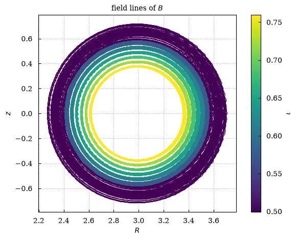

The traced ι against the exact one of the unperturbed field: away from the island they agree to better than one percent (trilinear interpolation of the direction field is second-order accurate in the grid spacing), and the plateau at ι = 1/2 is the island chain, where every line has the rational transform:

iota = lines.plasma.analysis.rotational_transform()
iota.swap_dims(line="eta1_start").plasma.plot.lineout(
    reference=lambda eta1: iota_exact(0.1 + 0.9 * eta1)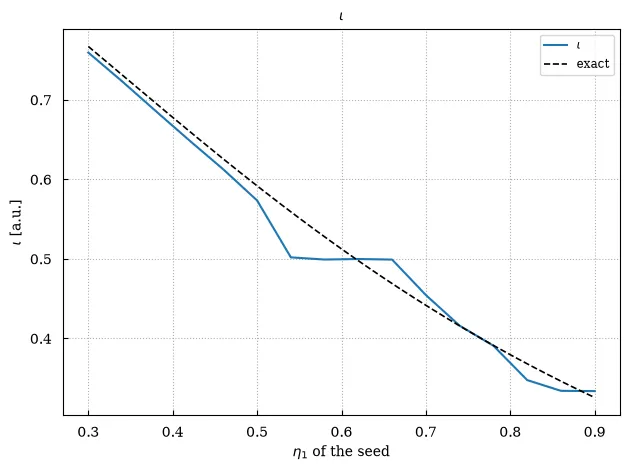
)

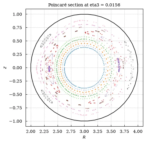
Poincaré sections

lines.plasma.plot.poincare()  # R against z, one color per line
lines.plasma.plot.poincare(coords="logical", color_by="iota")

Each line’s punctures trace a closed curve on a flux surface, a chain of m loops in an island, and a cloud where the field is chaotic. color_by takes "line" (the default, cycling), "iota" or "connection_length" (a color bar), "classification" (surface, island or chaotic, see below) or None; boundary= draws the outermost surface of any field with physical coordinates; max_lines= thins the plot.

The data behind this plot: lines.plasma.data.poincare() (or lines.plasma.analysis.poincare_section()) returns the punctures over (puncture, line) with their logical coordinates, x, y, z, R and the arc length s, and ι per line as a coordinate. poincare_section(angle=...) cuts another plane from the saved samples (as fine as the lines were saved; see stride).

B.plasma.plot.poincare(seeds=12, turns=100, t=-1) traces and plots in one call; the lines are in result.data["lines"].

The same plot with Plotly

The same call with backend="plotly": an interactive figure with the same data, fits and labels (see Interactive plots with Plotly).

lines.plasma.plot.poincare(backend="plotly")

Loading interactive chart…

Islands

# 0 surface, 1 island, 2 chaotic
codes = lines.plasma.analysis.classify_field_lines()
chains = lines.plasma.analysis.islands()
lines.plasma.plot.poincare(color_by="classification", islands=True)

classify_field_lines is a heuristic on the punctures of each line. Its rotational transform picks the lowest-order rational n/m within the trace’s resolution; the punctures are folded into one island by ψ = m θ mod period. Successive punctures of a line on a surface keep advancing in ψ (rotation), while those of a line inside an island turn back (libration about the O-point): a line whose accumulated ψ advance never spans a full period is in an island. Otherwise the punctures sorted by the poloidal angle should trace a smooth curve, the flux surface; large radial jumps between neighbours mean a chaotic line. A line whose punctures spread less than half a radial grid cell is a surface regardless.

islands groups the island lines by their rational and estimates each chain’s width: the radial extent of its widest island orbit, the one traced closest to the separatrix (so seed densely across a chain; one traced only near its O-point is underestimated). It returns a Dataset over chain with n, m, width (in the radial logical coordinate), width_physical, center, lines and the poloidal angle of one O-point. islands=True on the plot labels each chain with its n/m and width near an O-point.

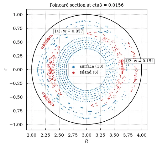
Trace long enough: a line inside an island must complete at least half a libration to be told from a surface, and a surface whose ι is closer to a rational than one over the number of transits passes as an island.

Open field lines: connection lengths and footprints

Where field lines leave the grid (a bounded radial direction, the ends of a torus sector), the connection length is the arc length from a point to the wall in both directions:

edge = B.plasma.analysis.field_lines(
    seeds={
        "eta1": 0.98,
        "eta2": np.linspace(0, 1, 48),
        "eta3": np.linspace(0, 1, 32),
    },
    direction="both",
    turns=50,
    t=-1,
)
edge.plasma.plot.connection_length()  # over the seed grid, log scale
# where the lines hit, colored by connection length
edge.plasma.plot.footprint()

With direction="both" each seed gives two lines (the coordinates seed and direction tell them apart) and connection_length is the sum of both exit lengths, NaN while a line has not left the grid within what was traced. edge.plasma.analysis.footprint() returns the exit points over line (NaN for confined lines); edge.plasma.analysis.seed_grid("connection_length") the map over the two seed coordinates, when the seeds form a grid, as a 2-D array any slice plot draws.

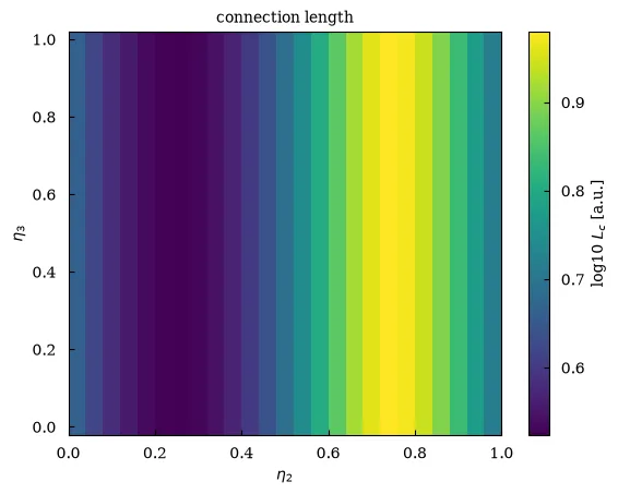
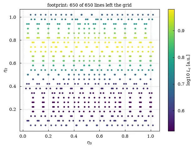
The figures use a periodic slab with B = (0.2 + 0.1 sin 2πη₂, 0, 1): the lines leave through the x faces, further along where the lean is smallest.

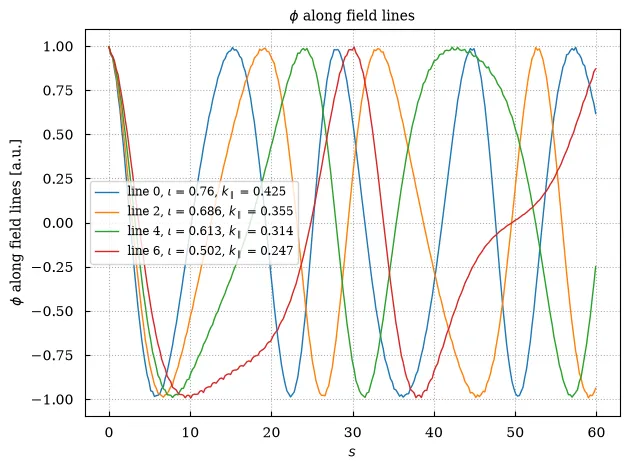
A field along the lines

along = phi.plasma.analysis.sample_along(lines)  # (t, s, line)
phi.plasma.plot.along_field_lines(lines, k_parallel=True, t=-1)
k_par = phi.plasma.analysis.parallel_wavenumber(lines=lines)

sample_along interpolates a scalar field trilinearly along the traced lines, keeping the field’s other dimensions; along.isel(line=0).plasma.plot.slice(x="s", y="t") is then a space-time map along one field line. parallel_wavenumber takes the peak of each line’s power spectrum over s (or counts zero crossings with method="crossings"); compare it with theory.waves.parallel_wavenumber, (n + m/q)/R₀ for a mode (m, n) in a cylinder. Here a mode cos(3θ − φ) along lines of different ι:

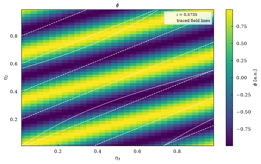
A flux surface, unfolded

phi.plasma.plot.surface_map(eta1=0.5, t=-1, iota=0.65, count=6)
boozer.mod_B.plasma.plot.surface_map(rho=0.5, iota=boozer.iota, count=8)
phi.plasma.plot.surface_map(eta1=0.5, t=-1, lines=lines.isel(line=[3]))

surface_map is a slice at one radius over the toroidal and poloidal angles, with field lines on it. In straight-field-line angles (GVEC’s Boozer or PEST angles) field lines are straight, θ = θ₀ + ι ζ: iota= draws count of them, a number or a profile over the radius, interpolated at the surface. On any grid, lines= draws traced lines over the angles as they are (the first two transits by default, turns=). A line that leaves the plot through a periodic edge continues from the opposite one.

Functions

The plain functions behind these methods, for arrays from anywhere, are in plasma_plots.fieldlines (trace_field_lines, poincare_section, rotational_transform, classify_field_lines, islands, footprint, seed_grid, sample_along, parallel_wavenumber) and plasma_plots.fieldline_plots (plot_poincare, plot_field_lines, plot_footprint, plot_connection_length, plot_along_field_lines, plot_surface_map).