LaTeX figures with TikZ

Every still plot that plasma-plots draws with Matplotlib can also be TikZ code, for a LaTeX document: pass backend="tikz". The figure is a pgfplots tikzpicture whose text is typeset by LaTeX, in the fonts of your document, and whose lines, markers and fits stay vector graphics you can still edit in the source.

pip install "plasma-plots[tikz]"    # maxplotlib, which does the conversion, and tikzfigure

Compiling the figures (.pdf, .png) needs pdflatex, as part of any TeX distribution.

One keyword

result = energy.plasma.plot.timeseries(
    fit=(0.0, 2.0), title="Field energy growth", backend="tikz"
)
result.save("energy.tikz")  # the tikzpicture, to \input in your paper
result.save("energy.tex")  # a standalone LaTeX document
result.save("energy.pdf")  # compiled with pdflatex; also .png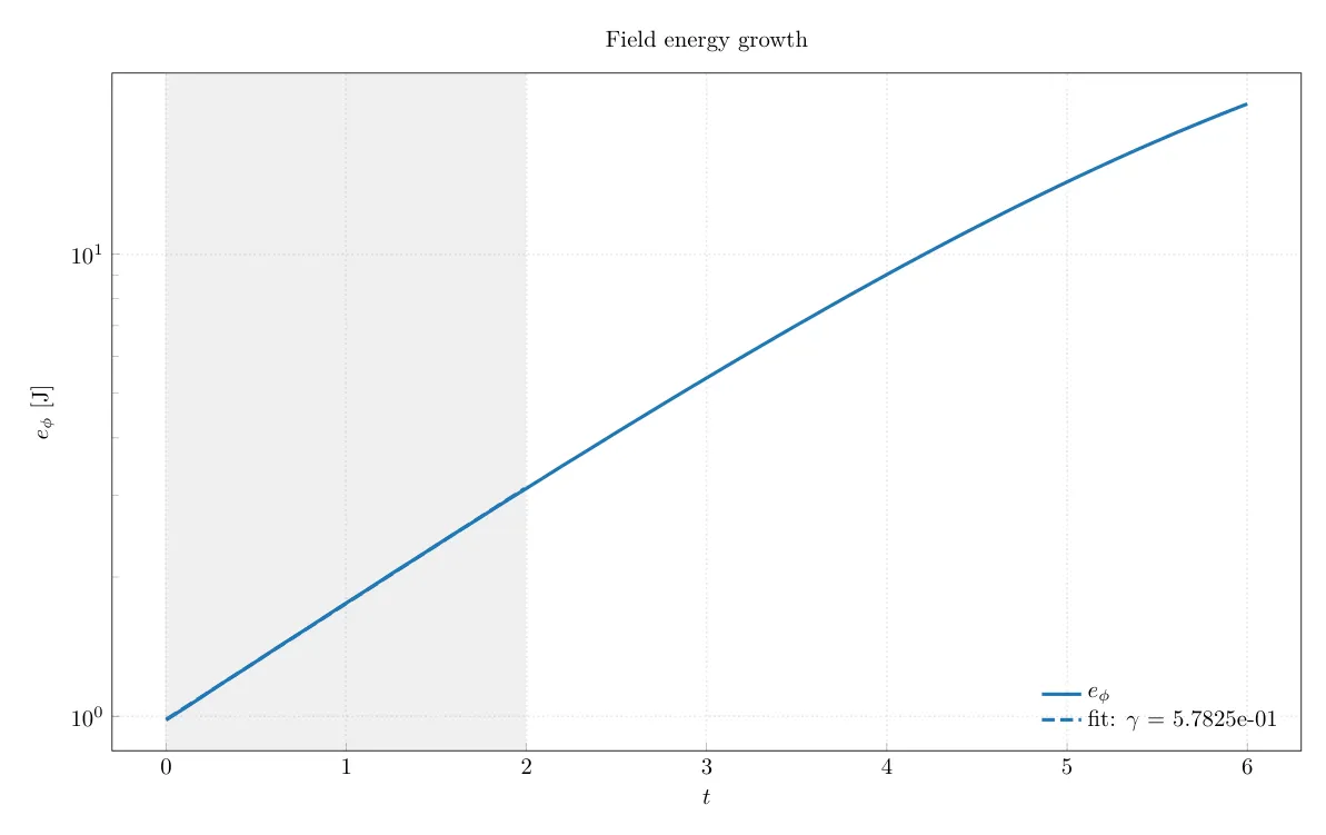

The TikZ version is the Matplotlib plot converted, not a second implementation. The plot is drawn with Matplotlib as usual, off screen, and maxplotlib converts the finished figure into a tikzfigure figure of pgfplots axes. Every panel is an axis at the place and size it has in the Matplotlib figure, with its limits, log scales, labels, title, ticks, grid, legend and colorbar. So the selection by keyword, the options, fit_results and data all stay the same:

result.fit_results[0].rate  # the same fit as with Matplotlib
result.fig  # a tikzfigure.TikzFigure
print(result.fig.generate_tikz())  # the code

\begin{tikzpicture}
    \definecolor{mpl1F77B4}{HTML}{1F77B4}
    \begin{axis}[scale only axis, at={(0.74in,0.58in)}, width=7.04in, height=4.05in,
        ymode=log, xlabel=$t$, ylabel={$e_\phi$ [J]}, title=Field energy growth, ...]
        \addplot[draw=mpl1F77B4, line width=1.5pt, ...] coordinates {(0,0.981392) ...};
        \addplot[draw=mpl1F77B4, line width=1.5pt, dash pattern=on 5.55pt off 2.4pt, ...] ...;
        \addlegendimage{draw=mpl1F77B4, line width=1.5pt, solid, mark=none}
        \addlegendentry{$e_\phi$}
        ...
    \end{axis}
\end{tikzpicture}

Fields and colorbars

Slices, panels, spectra and other colormaps would be slow and memory hungry as pgfplots coordinates, so the meshes are images, rendered by Matplotlib at 300 dpi and placed in the axis with \addplot graphics; on a mapped grid too. Everything drawn over them (contour lines, the domain’s boundary, markers, fits, text) stays vector graphics, and the axis, its ticks and labels are pgfplots. A colorbar is an axis of its own: its colors are an image, its ticks and label text.

result = phi.plasma.plot.slice(x="eta1", y="eta2", t=-1, backend="tikz")
result.save("phi.tikz")  # writes phi.tikz and the images it refers to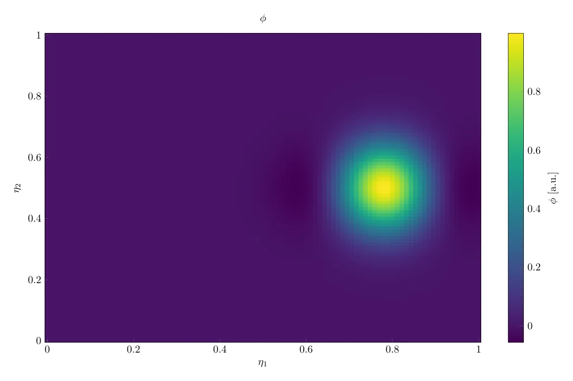

Saving as .tikz or .tex writes the images next to the file (as tikzfigure-<hash>.png), and the code refers to them by name. Keep them in the folder you compile from, or in a folder of \graphicspath. result.fig.files() lists them.

In your paper

The .tikz file is a tikzpicture. Load pgfplots in the preamble and \input it:

\usepackage{pgfplots}
\pgfplotsset{compat=newest}
...
\begin{figure}
  \centering
  \input{figures/energy.tikz}
  \caption{The field energy and its growth-rate fit.}
\end{figure}

The figure keeps the size the Matplotlib figure has (8 × 5 inches unless figsize says otherwise), and its text the Matplotlib font sizes, set with \fontsize. For a column of a paper, draw the plot at the size it will have in print, e.g. figsize=(3.4, 2.4), rather than scaling the tikzpicture: then the text has the size of the caption around it.

Text is converted from Matplotlib’s: mathtext ($\omega/\omega_{ci}$) is LaTeX math as it is, plain text is escaped (_, %, & are literal, as in Matplotlib), and Unicode symbols such as ω or ° become math. LaTeX math that Matplotlib’s mathtext does not know works too, since LaTeX typesets it.

For every plot at once, and composed figures

import plasma_plots

plasma_plots.set_backend("tikz")  # every plot from now on
out.plot.energies().save("energies.tikz")

plasma_plots.figure composes several plots into one TikZ figure, converted once at the end of the block:

with plasma_plots.figure(2, 1, sharex=True, backend="tikz") as fig:
    energy.plasma.plot.timeseries(fit=(0.0, 2.0), ax=fig[0])
    total.plasma.analysis.drift().plasma.plot.timeseries(logy=False, ax=fig[1])
fig.save("energies.tikz")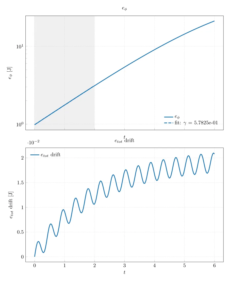

The plotting functions (plasma_plots.plotting.plot_slice, …) return Matplotlib results, which convert with .to_tikz(), and any Matplotlib figure converts with plasma_plots.tikz_backend.to_tikz(fig):

from plasma_plots.plotting import plot_slice

plot_slice(phi.isel(t=-1, eta3=0)).to_tikz().save("phi.tikz")

From the command line, an output ending in .tex or .tikz draws with backend=tikz:

plasma-plots plot sim_1 . energies -o energies.tikz

What becomes what

Matplotlib	TikZ
lines, fits, references, markers, error bars	\addplot, with the same colors, widths, dashes and marks
scatter plots of markers	\addplot[only marks], one per color and size
bars, spans (fit windows, bands), fills, polygons	closed \addplot paths
contour lines	\addplot per level
text, annotations, titles, labels	LaTeX text
meshes, images, filled contours, vector arrows	images in the axis
colorbars	an axis with its colors as an image
3-D axes (orbits in 3-D)	an image, with a TikzConversionWarning

TeX has limited memory, so a scatter plot of more than 2000 markers, a collection of more than 500 differently colored pieces and a line of more than 20000 points (after Matplotlib’s path simplification) are images too. plasma_plots.tikz_backend.OPTIONS sets the limits and the resolution of the images, e.g. OPTIONS["raster_dpi"] = 600; .to_tikz(raster_dpi=600) for one plot.

What has no TikZ version

• Animations and viewers: backend="tikz" raises TypeError; draw them with Matplotlib or Plotly, or a still of one frame with slice(t=...).
• The PyVista 3-D views (isosurface, slices_3d, glyphs, streamlines, volume, movie, orbits_3d) save screenshots; see 3-D views.
• ax=, which draws into a Matplotlib axes you made, cannot be combined with backend="tikz"; use plasma_plots.figure(..., backend="tikz") instead.