Spectral analysis
These tools transform any labeled array with a uniform t (or spatial)
coordinate. They run on demand, on the array you pass, so select a component,
region or time interval first when you don’t need the whole field. The
selected values are loaded into memory. Every tool is a method of
array.plasma.analysis (numbers and arrays) and most have a plot on
array.plasma.plot. The functions themselves live in plasma_plots.spectral
and plasma_plots.spectral_plots.
The examples on this page use a synthetic toroidal Alfvén eigenmode (TAE) in a sixth of a hollow torus. It has the geometry of Struphy’s TAE tutorial: r = 0.1 + 0.9 η₁, q = 1.71 + 0.16 r², R₀ = 10, and harmonics m = 10, 11 with n = 6. The coupled harmonics oscillate at the gap frequency ω_TAE ≈ 0.096 and grow slowly. A continuum-damped m = 10 oscillation sits at r = 0.8.
Conventions
Section titled “Conventions”- Every transform divides by the number of samples
N.time_fftis one-sided: itspowerdoubles the positive-frequency bins (but not the zero frequency, or the Nyquist bin of an evenN), sopower.sum("omega")equals the time mean square of the signal (Parseval). - Frequencies are angular, ω = 2πf, in units inverse to the
coordinate (
rad / sfor times in seconds). The spacing comes from the saved times, not the solver time step. Results recordfrequency_resolution= 2π/(NΔt),nyquist_frequency,sample_spacingandn_samplesin theirattrs. - The forward kernel is numpy’s exp(−iωt): exp(+iωt) appears at positive ω, and a mode exp(2πi(m η₂ + n η₃)) at (m, n).
- Grids must be uniform, finite and strictly increasing. Periodic spatial
grids that include both endpoints need
.plasma.analysis.drop_periodic_endpoint("eta2")beforefft(the mode tools do this themselves).
The dispersion plot (plot.dispersion()) is built on the same fft, so its
power follows these conventions too.
Power spectra
Section titled “Power spectra”# Dataset: coefficients, powerspectrum = phi.plasma.analysis.time_fft(detrend=True)# power per bin, averaged over spacespectrum.power.mean(("eta1", "eta2", "eta3"))# peak frequencies, refined below the bin spacingphi.plasma.analysis.spectral_peaks(n_peaks=2)
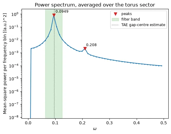
band = phi.plasma.analysis.filter_time( dims=("eta1", "eta2", "eta3"), pad_bins=3)phi.plasma.plot.power_spectrum( peaks=2, band=band, frequencies={"TAE gap-centre estimate": omega_tae})time_fft returns complex coefficients and one-sided power, with t
replaced by omega and every other dimension kept. detrend=True removes the
mean first, and window="hann" applies a periodic Hann taper. Neither is
compensated for in the power. spectral_peaks finds the strongest local maxima
and refines each frequency with a parabola through the log power of the peak
and its neighbors. That locates an off-bin frequency to a small fraction of a
bin, and also gives each peak’s half-power band.
The plot averages over every dimension but component, marks the peaks with
their refined frequencies, shades a filter band and draws reference lines:
Filtering a frequency band
Section titled “Filtering a frequency band”filter_time keeps the dominant peak’s half-power band and rebuilds the
signal from it. It sums the power over dims to pick one band shared by all
those points (default: every dimension except t and component), and never
keeps the zero frequency. pad_bins widens the band. That matters for a
growing or damped mode, whose line is broader than one bin:
band = phi.plasma.analysis.filter_time( dims=("eta1", "eta2", "eta3"), pad_bins=3)band.filtered # same dims, coordinates and units as phiband.spectrum # reduced power, dominant_frequency, omega_lo/hi, has_peakphi.plasma.plot.filtered(band, eta1=0.4, eta2=0.0, eta3=0.0)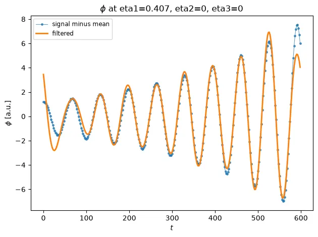
To choose the band yourself, e.g. a gap frequency read off a continuum plot,
use phi.plasma.analysis.band_filter(0.08, 0.11).
plasma_plots.spectral.inverse_time_fft(coefficients, template) inverts
time_fft coefficients. A finite record is treated as periodic, so leakage and
edge ringing are possible, and the strongest bin alone does not identify an
eigenfrequency.
Mode numbers
Section titled “Mode numbers”mode_spectrum Fourier-transforms along the periodic directions, poloidal
eta2 → m and toroidal eta3 → n by default, and keeps every other dimension:
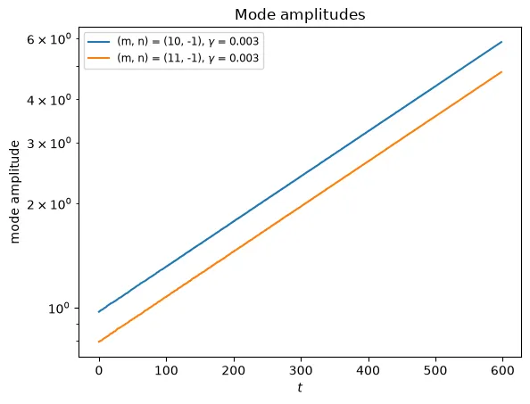
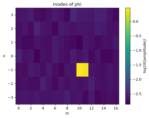
modes = phi.plasma.analysis.mode_spectrum() # complex, (t, eta1, m, n)# (t, eta1, mode), labels like "(10, -1)"amplitudes = modes.plasma.analysis.mode_amplitudes(top=4)phi.plasma.plot.mode_amplitudes(top=2, fit=(100, 500))phi.plasma.plot.mode_map(t=-1, m_range=(0, 16), n_range=(-3, 3))For a real field, mode_amplitudes merges each (m, n) with its conjugate
(−m, −n) and doubles the amplitude, so a field A cos(…) gives A. The
plot takes each mode’s maximum over the remaining dimensions (reduce="max",
here over radius) and fits growth rates. Both harmonics grow at the seeded
γ = 0.003:
relative=True divides each mode by the mean (the zero mode) at the same
point, as growth plots of an instability often show perturbations relative to
the background. For a ring whose edge ripples, take the amplitudes at the
interface, since a radial average would cancel the displacement:
n.sel(eta1=0.59, method="nearest").plasma.plot.mode_amplitudes( dims="eta2", names="m", relative=True, top=3, fit=(8, 20), eta3=0,)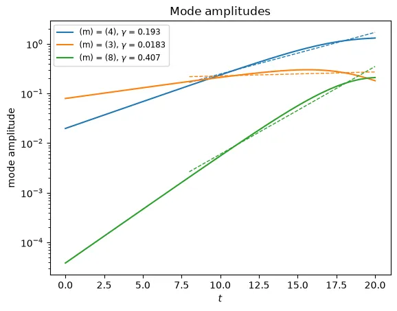
Struphy simulates a sector of the torus (tor_period=6 here), so n counts
periods per sector, and its sign follows the mapping’s orientation. n = −1
here is the full-torus |n| = 6.
Where each frequency lives
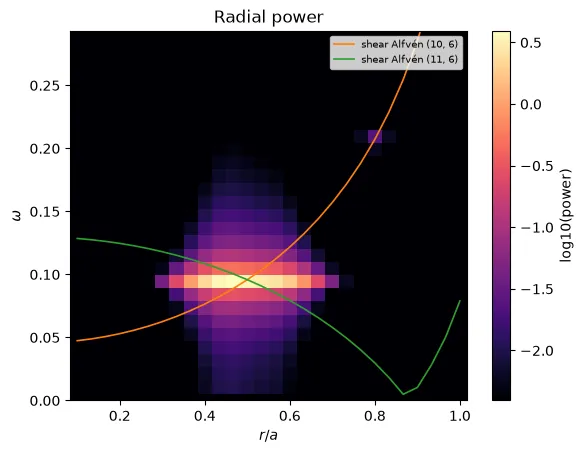
Section titled “Where each frequency lives”radial_power averages the power over the angles and plots it against
radius. x_of maps the logical eta1 to the minor radius, and continuum
draws the continuous spectra on top: any function omega(r, m, n), or
Struphy’s MhdContinousSpectraCylinder, as for the
continuous-spectrum plot:
phi.plasma.plot.radial_power( x_of=lambda eta1: 0.1 + 0.9 * eta1, xlabel="r/a", continuum=(alfven_continuum, [(10, 6), (11, 6)]), omega_max=0.3,)A global eigenmode is a horizontal ridge across the continuum crossing, where toroidal coupling opens the gap. A continuum-damped oscillation sits on a continuum curve, here the m = 10 branch at r = 0.8:
Continuous spectra
Section titled “Continuous spectra”plot_continuous_spectrum draws the continua on their own, one color per mode
and one line style per branch. spectrum is any function omega(x, *mode)
returning a mapping of branch names to frequencies, or one of Struphy’s
analytic continua, which give the shear-Alfvén and slow-sound branches of a
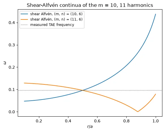
sheared slab or a cylinder. frequencies marks measured frequencies, to see
whether a mode sits in a gap or crosses a continuum, where it is damped:
from struphy.dispersion_relations.analytic import MhdContinousSpectraCylinderfrom plasma_plots.plotting import plot_continuous_spectrum
plot_continuous_spectrum(    MhdContinousSpectraCylinder(),    np.linspace(0.05, 1, 300),    [(10, 6), (11, 6)],    frequencies={"measured TAE frequency": omega},    xlabel="r",)
Here, with the uncoupled continua of the synthetic TAE, the measured frequency passes through the crossing of the m = 10 and 11 branches, where toroidal coupling opens the gap:
prepare_continuous_spectrum returns the curves as a (mode, branch, x)
array without plotting them.
Eigenfunctions
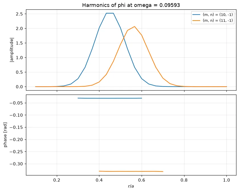
Section titled “Eigenfunctions”mode_structure(omega) gives the complex amplitude of the oscillation at one
exact frequency at every point. abs() of it is the eigenfunction’s amplitude
and np.angle() its phase. The frequency isn’t limited to FFT bins: use a
refined peak frequency. mode_profiles combines it with mode_spectrum to show
the radial profile of each harmonic:
omega = float( phi.plasma.analysis.spectral_peaks(n_peaks=1, window="hann").omega_refined[ 0 ])# complex, (eta1, eta2, eta3)structure = phi.plasma.analysis.mode_structure(omega)phi.plasma.plot.mode_profiles(omega, x_of=lambda eta1: 0.1 + 0.9 * eta1, top=2)The m = 10 and m = 11 harmonics peak either side of r* = 0.5, and their phases are flat and locked together. The coupled harmonics of a global mode oscillate together like this, whereas continuum-damped structure mixes its phase across radius:
Without a frequency, mode_profiles shows the harmonics’ amplitudes at one
time. scale multiplies the mode numbers, so scale=(1, 6) labels a sixth of
a torus (tor_period=6) with full-torus toroidal mode numbers:
phi.plasma.plot.mode_profiles( t=-1, scale=(1, 6), x_of=lambda eta1: 0.1 + 0.9 * eta1, top=2)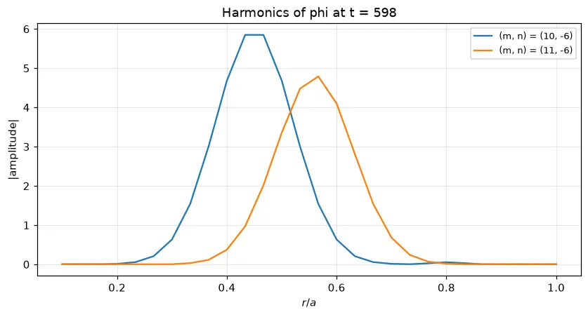
The energy in a filtered mode comes from energies from fields.
The filtered mode, drawn in its torus sector with the 3-D views:
band.filtered.isel(t=-1).plasma.plot.slices_3d( cuts={"eta3": [0, 0.5, 1], "eta1": 0.44}, cmap="RdBu_r")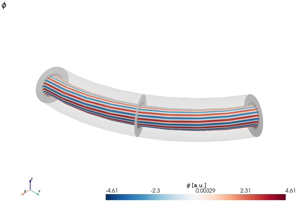
Drag to rotate, scroll to zoom, shift-drag to pan.Open in a new tab
Frequency and growth from a short record
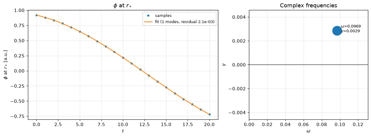
Section titled “Frequency and growth from a short record”The TAE period is about 66 time units. A run to t = 20 covers a third of it,
and the FFT’s first nonzero bin, 2π/21 ≈ 0.30, lies above ω_TAE. Zero
padding would only interpolate. matrix_pencil
fits a sum of growing or damped oscillations directly instead: the frequency
and growth (or damping) rate of each mode, with no bin limit:
# omega, gamma, amplitude, phase per modefit = probe.plasma.analysis.matrix_pencil(n_modes=1)probe.plasma.plot.pencil_fit(n_modes=1)From 21 noisy samples it finds ω = 0.097 and γ = 0.0028
(seeded: 0.096 and 0.003). The residual in fit.attrs checks the fit. Use as
few modes as the signal needs, since extra modes fit noise. For a real signal,
n_modes counts oscillations, each a conjugate pair.
An energy is quadratic in the field, so it oscillates at twice the wave
frequency, around a trend when the wave grows or decays. spectral_peaks
takes a polynomial degree as detrend for that case:
en_U.plasma.analysis.spectral_peaks(detrend=2, window="hann") puts the peak
at 2ω.
Changing frequencies: spectrograms
Section titled “Changing frequencies: spectrograms”spectrogram(length=...) computes power spectra in sliding windows. length
and step are sample counts (integers) or time spans (floats). It shows a
frequency that drifts, such as an energetic-particle mode chirping down, next
to a steady one. It also separates an initial transient from a persistent
oscillation:
signal.plasma.plot.spectrogram(length=200.0, step=10.0, omega_max=0.45)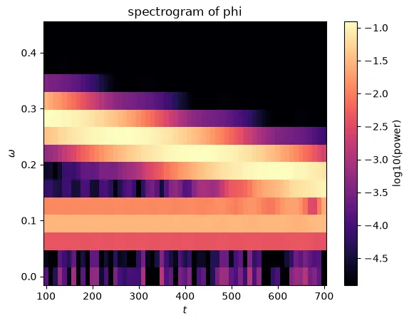
The resolution is 2π divided by the window length: a longer window resolves frequency better and time worse.
Phase between two fields
Section titled “Phase between two fields”cross_spectrum(other) gives the phase by which other leads the array at
each frequency. With dims, the points become an ensemble and coherence
(between 0 and 1) measures how consistently that phase holds across them. In a
standing shear-Alfvén wave, velocity and magnetic perturbation exchange energy
a quarter period apart:
u.plasma.plot.cross_spectrum(b, dims="eta3", omega_max=1.5)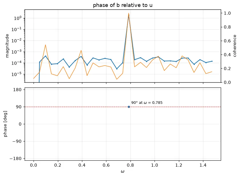
Whole runs
Section titled “Whole runs”out.analysis takes a product name or an array. It mirrors the
postprocessing-fft Output API:
out.analysis.time_fft("mhd/velocity")out.analysis.fft(field, dim="eta2")out.analysis.filter_time(field, dims=("eta1", "eta2"), pad_bins=2)out.analysis.mode_spectrum("mhd/velocity")See plasma_plots.spectral and
plasma_plots.spectral_plots for every
function and option.