Tokamak X-Point with Parametric TikZ Plots
This tutorial builds on Mathematical Expressions and focuses on the plain TikZ plotting API by building up to a stylized tokamak X-point / separatrix drawing in a poloidal cross-section.
The goal is not to derive a full equilibrium solver inside TikZ. Instead, the point is to show how declared PGF functions, parametric expressions, and looped sampling can be combined to produce the kind of contour structure you see in an X-point divertor configuration.
Along the way we will use:
fig.plot(...)for a single sampled plotloop.plot(...)for families of curves- callable objects returned by
fig.declare_function(...) func(name, ...)when you still want the string-based interface
These plots are regular TikZ \draw ... plot(...) commands, not
pgfplots axis plots.
from tikzfigure import TikzFigure, colorsfrom tikzfigure.math import Var, cos, exp, func, ln, sinA first sampled curve
Section titled “A first sampled curve”The simplest case is a regular function graph. Here fig.plot(...)
samples a single expression over a domain. This is the basic building
block behind all of the more complicated flux-surface-like contours
later in the tutorial.
fig = TikzFigure(figsize=(8, 4))
x = Var("x")
fig.draw([(-2.4, 0), (2.4, 0)], color="gray")fig.draw([(0, -0.8), (0, 0.8)], color="gray")fig.plot(    sin(90 * x) / 2,    variable="x",    domain=(-2, 2),    samples=120,    smooth=True,    options=[colors.blue],)
fig.show()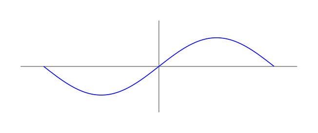
Show Tikz code
print(fig)% --------------------------------------------- %% Tikzfigure generated by tikzfigure v0.3.1 %% https://github.com/max-models/tikzfigure %% --------------------------------------------- %\begin{tikzpicture} \draw[color=gray] (-2.4, 0) to (2.4, 0); \draw[color=gray] (0, -0.8) to (0, 0.8); \draw[blue, smooth, variable=\x, domain=-2:2, samples=120] plot ({\x}, {(sin((90 * \x)) / 2)});\end{tikzpicture}print(fig.generate_standalone())\documentclass[border=10pt]{standalone}\PassOptionsToPackage{dvipsnames,svgnames,x11names}{xcolor}\usepackage{tikz}\usepackage{pgfplots}\pgfplotsset{compat=newest}\usepgfplotslibrary{groupplots}\usetikzlibrary{arrows.meta}\begin{document}% --------------------------------------------- %% Tikzfigure generated by tikzfigure v0.3.1 %% https://github.com/max-models/tikzfigure %% --------------------------------------------- %\begin{tikzpicture} \draw[color=gray] (-2.4, 0) to (2.4, 0); \draw[color=gray] (0, -0.8) to (0, 0.8); \draw[blue, smooth, variable=\x, domain=-2:2, samples=120] plot ({\x}, {(sin((90 * \x)) / 2)});\end{tikzpicture}
\end{document}When only one expression is passed, TikZ uses the sampling variable as the x-coordinate and the expression as the y-coordinate.
Declaring a custom shaping function
Section titled “Declaring a custom shaping function”You can declare helper functions once and reuse them in later plots. For this tutorial we will use a hyperbolic-tangent-like shaping function that will later help us bend contours into an X-point geometry.
fig = TikzFigure(figsize=(8, 4))
th = fig.declare_function(    "th",    "x",    (1 - exp(-2 * Var("x"))) / (1 + exp(-2 * Var("x"))),)
x = Var("x")
fig.draw([(-3.4, 0), (3.4, 0)], color="gray")fig.draw([(0, -1.1), (0, 1.1)], color="gray")fig.plot(    th(x),    variable="x",    domain=(-3, 3),    samples=150,    smooth=True,    options=[colors.Azure4],    line_width="0.8pt",)
fig.show()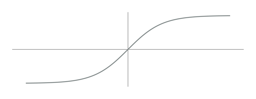
Show Tikz code
print(fig)% --------------------------------------------- %% Tikzfigure generated by tikzfigure v0.3.1 %% https://github.com/max-models/tikzfigure %% --------------------------------------------- %\begin{tikzpicture} \pgfkeys{/pgf/declare function={th(\x) = ((1 - exp((-2 * \x))) / (1 + exp((-2 * \x))));}} \draw[color=gray] (-3.4, 0) to (3.4, 0); \draw[color=gray] (0, -1.1) to (0, 1.1); \draw[Azure4, smooth, line width=0.8pt, variable=\x, domain=-3:3, samples=150] plot ({\x}, {th(\x)});\end{tikzpicture}print(fig.generate_standalone())\documentclass[border=10pt]{standalone}\PassOptionsToPackage{dvipsnames,svgnames,x11names}{xcolor}\usepackage{tikz}\usepackage{pgfplots}\pgfplotsset{compat=newest}\usepgfplotslibrary{groupplots}\usetikzlibrary{arrows.meta}\begin{document}% --------------------------------------------- %% Tikzfigure generated by tikzfigure v0.3.1 %% https://github.com/max-models/tikzfigure %% --------------------------------------------- %\begin{tikzpicture} \pgfkeys{/pgf/declare function={th(\x) = ((1 - exp((-2 * \x))) / (1 + exp((-2 * \x))));}} \draw[color=gray] (-3.4, 0) to (3.4, 0); \draw[color=gray] (0, -1.1) to (0, 1.1); \draw[Azure4, smooth, line width=0.8pt, variable=\x, domain=-3:3, samples=150] plot ({\x}, {th(\x)});\end{tikzpicture}
\end{document}The object returned by fig.declare_function(...) is callable, so the
most natural way to use it is th(x). The older func("th", x) style
still works when you want it.
Your first closed flux-surface-like curve
Section titled “Your first closed flux-surface-like curve”If you pass both x and y expressions, the plot becomes parametric.
This is the key step from ordinary function graphs to closed
magnetic-surface-like contours.
fig = TikzFigure(figsize=(7, 7))
fig.variable("scale", 1.25)fig.variable("radius", 1.6)arcth = fig.declare_function(    "arcth",    "x",    0.5 * ln((1 + Var("x")) / (1 - Var("x"))),)th = fig.declare_function(    "th",    "x",    (1 - exp(-2 * Var("x"))) / (1 + exp(-2 * Var("x"))),)
theta = Var("theta")radius = Var("radius")
curve_x = Var("scale") * arcth(th(radius) * cos(theta))curve_y = Var("scale") * arcth(th(radius) * sin(theta))
fig.plot(    curve_x,    curve_y,    variable="theta",    domain=(0, 360),    samples=140,    smooth=True,    options=[colors.Azure4],)
fig.show()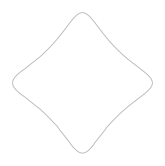
Show Tikz code
print(fig)% --------------------------------------------- %% Tikzfigure generated by tikzfigure v0.3.1 %% https://github.com/max-models/tikzfigure %% --------------------------------------------- %\begin{tikzpicture} \pgfmathsetmacro{\scale}{1.25} \pgfmathsetmacro{\radius}{1.6} \pgfkeys{/pgf/declare function={arcth(\x) = (0.5 * ln(((1 + \x) / (1 - \x))));}} \pgfkeys{/pgf/declare function={th(\x) = ((1 - exp((-2 * \x))) / (1 + exp((-2 * \x))));}} \draw[Azure4, smooth, variable=\theta, domain=0:360, samples=140] plot ({(\scale * arcth((th(\radius) * cos(\theta))))}, {(\scale * arcth((th(\radius) * sin(\theta))))});\end{tikzpicture}print(fig.generate_standalone())\documentclass[border=10pt]{standalone}\PassOptionsToPackage{dvipsnames,svgnames,x11names}{xcolor}\usepackage{tikz}\usepackage{pgfplots}\pgfplotsset{compat=newest}\usepgfplotslibrary{groupplots}\usetikzlibrary{arrows.meta}\begin{document}% --------------------------------------------- %% Tikzfigure generated by tikzfigure v0.3.1 %% https://github.com/max-models/tikzfigure %% --------------------------------------------- %\begin{tikzpicture} \pgfmathsetmacro{\scale}{1.25} \pgfmathsetmacro{\radius}{1.6} \pgfkeys{/pgf/declare function={arcth(\x) = (0.5 * ln(((1 + \x) / (1 - \x))));}} \pgfkeys{/pgf/declare function={th(\x) = ((1 - exp((-2 * \x))) / (1 + exp((-2 * \x))));}} \draw[Azure4, smooth, variable=\theta, domain=0:360, samples=140] plot ({(\scale * arcth((th(\radius) * cos(\theta))))}, {(\scale * arcth((th(\radius) * sin(\theta))))});\end{tikzpicture}
\end{document}Now the sampling variable is \theta, and both coordinates are computed
from it. You can think of \theta here as a poloidal-angle-like
parameter tracing a single closed contour.
Building a family of nested flux surfaces
Section titled “Building a family of nested flux surfaces”The same parametric expression becomes much more interesting when
combined with fig.loop(...).
fig = TikzFigure(figsize=(8, 8))
fig.variable("scale", 1.25)arcth = fig.declare_function(    "arcth",    "x",    0.5 * ln((1 + Var("x")) / (1 - Var("x"))),)th = fig.declare_function(    "th",    "x",    (1 - exp(-2 * Var("x"))) / (1 + exp(-2 * Var("x"))),)
theta = Var("theta")
with fig.loop("i", range(21)) as i:    radius = 0.2 * i    curve_x = Var("scale") * arcth(th(radius) * cos(theta))    curve_y = Var("scale") * arcth(th(radius) * sin(theta))    fig.plot(        curve_x,        curve_y,        variable="theta",        domain=(0, 360),        samples=100,        smooth=True,        options=[colors.Azure4],    )
fig.show()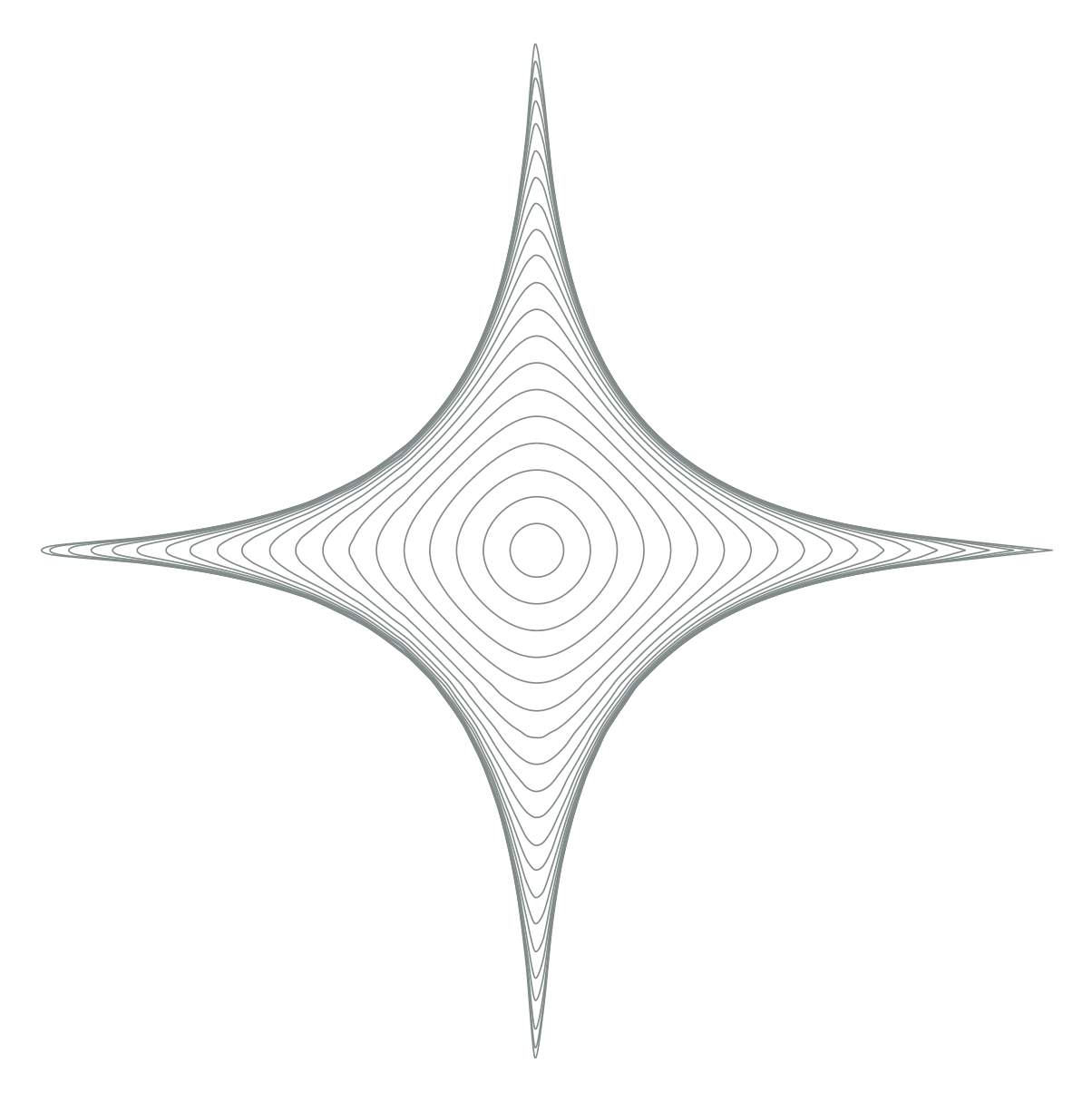
Show Tikz code
print(fig)% --------------------------------------------- %% Tikzfigure generated by tikzfigure v0.3.1 %% https://github.com/max-models/tikzfigure %% --------------------------------------------- %\begin{tikzpicture} \pgfmathsetmacro{\scale}{1.25} \pgfkeys{/pgf/declare function={arcth(\x) = (0.5 * ln(((1 + \x) / (1 - \x))));}} \pgfkeys{/pgf/declare function={th(\x) = ((1 - exp((-2 * \x))) / (1 + exp((-2 * \x))));}} \foreach \i in {0,1,...,20}{ \draw[Azure4, smooth, variable=\theta, domain=0:360, samples=100] plot ({(\scale * arcth((th((0.2 * \i)) * cos(\theta))))}, {(\scale * arcth((th((0.2 * \i)) * sin(\theta))))}); }\end{tikzpicture}print(fig.generate_standalone())\documentclass[border=10pt]{standalone}\PassOptionsToPackage{dvipsnames,svgnames,x11names}{xcolor}\usepackage{tikz}\usepackage{pgfplots}\pgfplotsset{compat=newest}\usepgfplotslibrary{groupplots}\usetikzlibrary{arrows.meta}\begin{document}% --------------------------------------------- %% Tikzfigure generated by tikzfigure v0.3.1 %% https://github.com/max-models/tikzfigure %% --------------------------------------------- %\begin{tikzpicture} \pgfmathsetmacro{\scale}{1.25} \pgfkeys{/pgf/declare function={arcth(\x) = (0.5 * ln(((1 + \x) / (1 - \x))));}} \pgfkeys{/pgf/declare function={th(\x) = ((1 - exp((-2 * \x))) / (1 + exp((-2 * \x))));}} \foreach \i in {0,1,...,20}{ \draw[Azure4, smooth, variable=\theta, domain=0:360, samples=100] plot ({(\scale * arcth((th((0.2 * \i)) * cos(\theta))))}, {(\scale * arcth((th((0.2 * \i)) * sin(\theta))))}); }\end{tikzpicture}
\end{document}Each loop iteration gives TikZ a different integer value of \i.
Because the context variable i now behaves like that TikZ variable
directly, you can derive the physical radius inside the block with
radius = 0.2 * i and then use the ordinary fig.plot(...) API inside
the loop body. That keeps the loop compact while still producing a whole
family of nested contours. In the tokamak picture, these read naturally
as flux surfaces moving outward from the core.
Adding the crossing family near the X-point
Section titled “Adding the crossing family near the X-point”Next, add the second family by keeping \theta fixed and varying \r.
Once both families are drawn, the contour structure starts to look like
the crossing geometry around an X-point.
fig = TikzFigure(figsize=(8, 8))
fig.variable("scale", 1.25)arcth = fig.declare_function(    "arcth",    "x",    0.5 * ln((1 + Var("x")) / (1 - Var("x"))),)th = fig.declare_function(    "th",    "x",    (1 - exp(-2 * Var("x"))) / (1 + exp(-2 * Var("x"))),)
theta = Var("theta")
with fig.loop("i", range(21)) as i:    radius = 0.2 * i    curve_x_loop = Var("scale") * arcth(th(radius) * cos(theta))    curve_y_loop = Var("scale") * arcth(th(radius) * sin(theta))    fig.plot(        curve_x_loop,        curve_y_loop,        variable="theta",        domain=(0, 360),        samples=100,        smooth=True,        options=[colors.Azure4],    )
with fig.loop("theta", range(0, 361, 9)) as theta:    r = Var("r")    curve_x_cross = Var("scale") * arcth(th(r) * cos(theta))    curve_y_cross = Var("scale") * arcth(th(r) * sin(theta))    fig.plot(        curve_x_cross,        curve_y_cross,        variable="r",        domain=(0, 4),        samples=15,        smooth=True,        options=[colors.Azure4],    )
fig.show()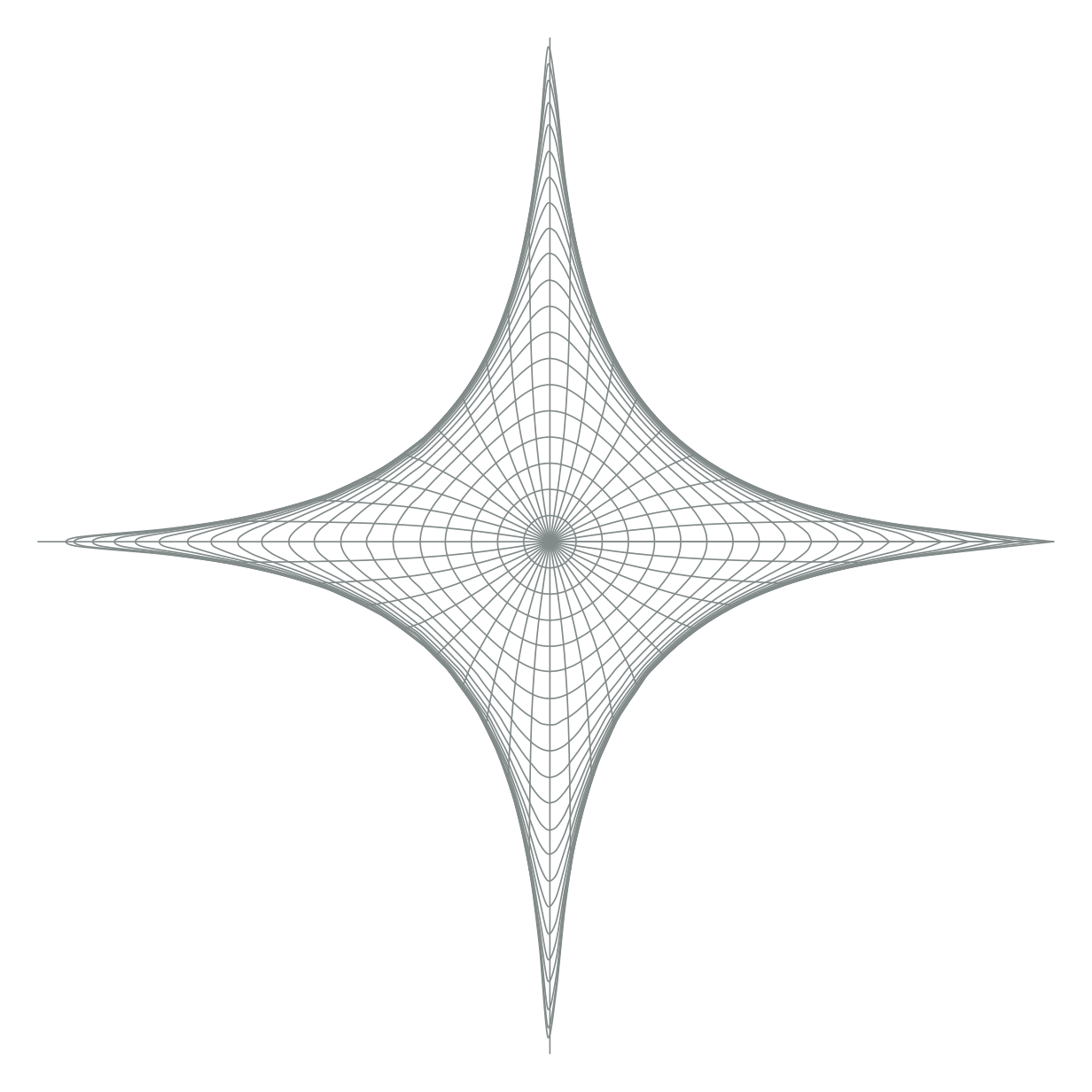
Show Tikz code
print(fig)% --------------------------------------------- %% Tikzfigure generated by tikzfigure v0.3.1 %% https://github.com/max-models/tikzfigure %% --------------------------------------------- %\begin{tikzpicture} \pgfmathsetmacro{\scale}{1.25} \pgfkeys{/pgf/declare function={arcth(\x) = (0.5 * ln(((1 + \x) / (1 - \x))));}} \pgfkeys{/pgf/declare function={th(\x) = ((1 - exp((-2 * \x))) / (1 + exp((-2 * \x))));}} \foreach \i in {0,1,...,20}{ \draw[Azure4, smooth, variable=\theta, domain=0:360, samples=100] plot ({(\scale * arcth((th((0.2 * \i)) * cos(\theta))))}, {(\scale * arcth((th((0.2 * \i)) * sin(\theta))))}); } \foreach \theta in {0,9,...,360}{ \draw[Azure4, smooth, variable=\r, domain=0:4, samples=15] plot ({(\scale * arcth((th(\r) * cos(\theta))))}, {(\scale * arcth((th(\r) * sin(\theta))))}); }\end{tikzpicture}print(fig.generate_standalone())\documentclass[border=10pt]{standalone}\PassOptionsToPackage{dvipsnames,svgnames,x11names}{xcolor}\usepackage{tikz}\usepackage{pgfplots}\pgfplotsset{compat=newest}\usepgfplotslibrary{groupplots}\usetikzlibrary{arrows.meta}\begin{document}% --------------------------------------------- %% Tikzfigure generated by tikzfigure v0.3.1 %% https://github.com/max-models/tikzfigure %% --------------------------------------------- %\begin{tikzpicture} \pgfmathsetmacro{\scale}{1.25} \pgfkeys{/pgf/declare function={arcth(\x) = (0.5 * ln(((1 + \x) / (1 - \x))));}} \pgfkeys{/pgf/declare function={th(\x) = ((1 - exp((-2 * \x))) / (1 + exp((-2 * \x))));}} \foreach \i in {0,1,...,20}{ \draw[Azure4, smooth, variable=\theta, domain=0:360, samples=100] plot ({(\scale * arcth((th((0.2 * \i)) * cos(\theta))))}, {(\scale * arcth((th((0.2 * \i)) * sin(\theta))))}); } \foreach \theta in {0,9,...,360}{ \draw[Azure4, smooth, variable=\r, domain=0:4, samples=15] plot ({(\scale * arcth((th(\r) * cos(\theta))))}, {(\scale * arcth((th(\r) * sin(\theta))))}); }\end{tikzpicture}
\end{document}The full X-point / separatrix sketch
Section titled “The full X-point / separatrix sketch”Now add a second pass with thicker red guide curves to highlight a few selected surfaces and the separatrix-like branches.
fig = TikzFigure(figsize=(9, 9))
fig.variable("scale", 1.25)arcth = fig.declare_function(    "arcth",    "x",    0.5 * ln((1 + Var("x")) / (1 - Var("x"))),)th = fig.declare_function(    "th",    "x",    (1 - exp(-2 * Var("x"))) / (1 + exp(-2 * Var("x"))),)
theta = Var("theta")
fine_radii = range(21)major_radii = range(5, 21, 5)fine_angles = range(0, 361, 9)major_angles = range(0, 360, 30)
with fig.loop("i", fine_radii) as i:    radius = 0.2 * i    curve_x_loop = Var("scale") * arcth(th(radius) * cos(theta))    curve_y_loop = Var("scale") * arcth(th(radius) * sin(theta))    fig.plot(        curve_x_loop,        curve_y_loop,        variable="theta",        domain=(0, 360),        samples=100,        smooth=True,        options=[colors.Azure4],    )
with fig.loop("theta", fine_angles) as theta:    r = Var("r")    curve_x_cross = Var("scale") * arcth(th(r) * cos(theta))    curve_y_cross = Var("scale") * arcth(th(r) * sin(theta))    fig.plot(        curve_x_cross,        curve_y_cross,        variable="r",        domain=(0, 4),        samples=15,        smooth=True,        options=[colors.Azure4],    )
with fig.loop("i", major_radii) as i:    radius = 0.2 * i    curve_x_loop = Var("scale") * arcth(th(radius) * cos(theta))    curve_y_loop = Var("scale") * arcth(th(radius) * sin(theta))    fig.plot(        curve_x_loop,        curve_y_loop,        variable="theta",        domain=(0, 360),        samples=120,        smooth=True,        options=[colors.Red3],        line_width="0.9pt",    )
with fig.loop("theta", major_angles) as theta:    r = Var("r")    curve_x_cross = Var("scale") * arcth(th(r) * cos(theta))    curve_y_cross = Var("scale") * arcth(th(r) * sin(theta))    fig.plot(        curve_x_cross,        curve_y_cross,        variable="r",        domain=(0, 4),        samples=25,        smooth=True,        options=[colors.Red3],        line_width="0.9pt",    )
fig.show()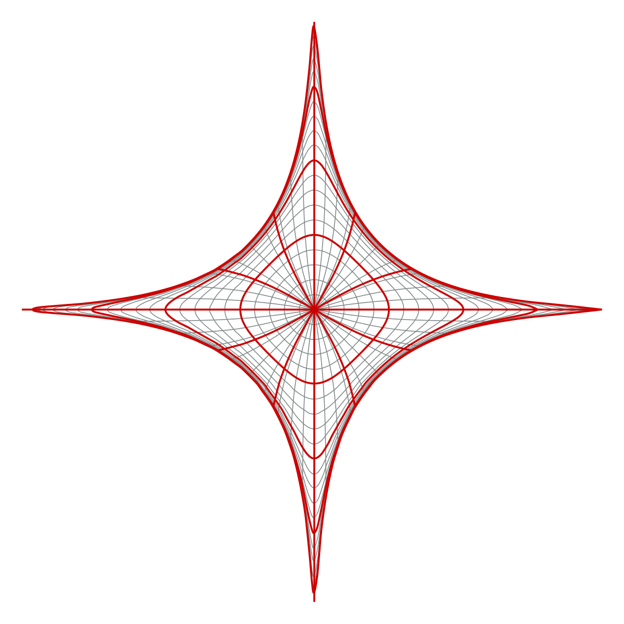
Show Tikz code
print(fig)% --------------------------------------------- %% Tikzfigure generated by tikzfigure v0.3.1 %% https://github.com/max-models/tikzfigure %% --------------------------------------------- %\begin{tikzpicture} \pgfmathsetmacro{\scale}{1.25} \pgfkeys{/pgf/declare function={arcth(\x) = (0.5 * ln(((1 + \x) / (1 - \x))));}} \pgfkeys{/pgf/declare function={th(\x) = ((1 - exp((-2 * \x))) / (1 + exp((-2 * \x))));}} \foreach \i in {0,1,...,20}{ \draw[Azure4, smooth, variable=\theta, domain=0:360, samples=100] plot ({(\scale * arcth((th((0.2 * \i)) * cos(\theta))))}, {(\scale * arcth((th((0.2 * \i)) * sin(\theta))))}); } \foreach \theta in {0,9,...,360}{ \draw[Azure4, smooth, variable=\r, domain=0:4, samples=15] plot ({(\scale * arcth((th(\r) * cos(\theta))))}, {(\scale * arcth((th(\r) * sin(\theta))))}); } \foreach \i in {5,10,...,20}{ \draw[Red3, smooth, line width=0.9pt, variable=\theta, domain=0:360, samples=120] plot ({(\scale * arcth((th((0.2 * \i)) * cos(\theta))))}, {(\scale * arcth((th((0.2 * \i)) * sin(\theta))))}); } \foreach \theta in {0,30,...,330}{ \draw[Red3, smooth, line width=0.9pt, variable=\r, domain=0:4, samples=25] plot ({(\scale * arcth((th(\r) * cos(\theta))))}, {(\scale * arcth((th(\r) * sin(\theta))))}); }\end{tikzpicture}print(fig.generate_standalone())\documentclass[border=10pt]{standalone}\PassOptionsToPackage{dvipsnames,svgnames,x11names}{xcolor}\usepackage{tikz}\usepackage{pgfplots}\pgfplotsset{compat=newest}\usepgfplotslibrary{groupplots}\usetikzlibrary{arrows.meta}\begin{document}% --------------------------------------------- %% Tikzfigure generated by tikzfigure v0.3.1 %% https://github.com/max-models/tikzfigure %% --------------------------------------------- %\begin{tikzpicture} \pgfmathsetmacro{\scale}{1.25} \pgfkeys{/pgf/declare function={arcth(\x) = (0.5 * ln(((1 + \x) / (1 - \x))));}} \pgfkeys{/pgf/declare function={th(\x) = ((1 - exp((-2 * \x))) / (1 + exp((-2 * \x))));}} \foreach \i in {0,1,...,20}{ \draw[Azure4, smooth, variable=\theta, domain=0:360, samples=100] plot ({(\scale * arcth((th((0.2 * \i)) * cos(\theta))))}, {(\scale * arcth((th((0.2 * \i)) * sin(\theta))))}); } \foreach \theta in {0,9,...,360}{ \draw[Azure4, smooth, variable=\r, domain=0:4, samples=15] plot ({(\scale * arcth((th(\r) * cos(\theta))))}, {(\scale * arcth((th(\r) * sin(\theta))))}); } \foreach \i in {5,10,...,20}{ \draw[Red3, smooth, line width=0.9pt, variable=\theta, domain=0:360, samples=120] plot ({(\scale * arcth((th((0.2 * \i)) * cos(\theta))))}, {(\scale * arcth((th((0.2 * \i)) * sin(\theta))))}); } \foreach \theta in {0,30,...,330}{ \draw[Red3, smooth, line width=0.9pt, variable=\r, domain=0:4, samples=25] plot ({(\scale * arcth((th(\r) * cos(\theta))))}, {(\scale * arcth((th(\r) * sin(\theta))))}); }\end{tikzpicture}
\end{document}This final figure uses the exact same ingredients as the earlier steps: declared functions, composable expressions, sampled plots, and loops. The result is a stylized tokamak X-point drawing with a separatrix-like structure, built entirely from plain TikZ plots.