Mathematical Expressions
tikzfigure includes a math module that lets you build PGF
mathematical expressions in Python. This is useful for creating
parametric or symbolic geometries without manually writing TikZ syntax.
Instead of hardcoding coordinates like (1.5, 2.0), you can write
(sin(60), cos(60)) or (Var("radius") * 2, Var("angle")) — all as
Python code, with full composability and operator support.
This tutorial covers:
- Building expressions with functions and operators
- Using expressions as node coordinates
- Using expressions in variables
- Composing complex expressions
- Available PGF functions and constants
from tikzfigure import TikzFigure, arrowsfrom tikzfigure.math import sin, cos, sqrt, Var, pi, max, minYour first expression
Section titled “Your first expression”Any PGF math function is available as a Python function. Calling it
returns an Expr object that knows how to render itself into valid PGF
syntax.
# Basic expressionsexpr1 = sin(60)expr2 = cos(45)expr3 = sqrt(2)
print(f"sin(60) → {expr1}")print(f"cos(45) → {expr2}")print(f"sqrt(2) → {expr3}")
sin(60) → sin(60)cos(45) → cos(45)sqrt(2) → sqrt(2)When you pass an Expr to a TikZ method, it’s automatically converted
to a string via __str__.
Using expressions as node coordinates
Section titled “Using expressions as node coordinates”Any coordinate parameter (x, y, or in a tuple) accepts expressions:
fig = TikzFigure(figsize=(10, 8))
# Place nodes at trigonometric coordinatesfig.node(    (sin(0), cos(0)),    label="P0",    content="(sin 0°, cos 0°)",    fill="red!30",    shape="circle",)fig.node(    (sin(45), cos(45)),    label="P45",    content="(sin 45°, cos 45°)",    fill="blue!30",    shape="circle",)fig.node(    (sin(90), cos(90)),    label="P90",    content="(sin 90°, cos 90°)",    fill="green!30",    shape="circle",)fig.node(    (sin(180), cos(180)),    label="P180",    content="(sin 180°, cos 180°)",    fill="yellow!30",    shape="circle",)
# Draw a path using expressionsfig.draw(    [        (sin(0), cos(0)),        (sin(45), cos(45)),        (sin(90), cos(90)),        (sin(180), cos(180)),    ],    arrows=arrows.forward,    color="gray",    line_width=1.5,)
fig.show()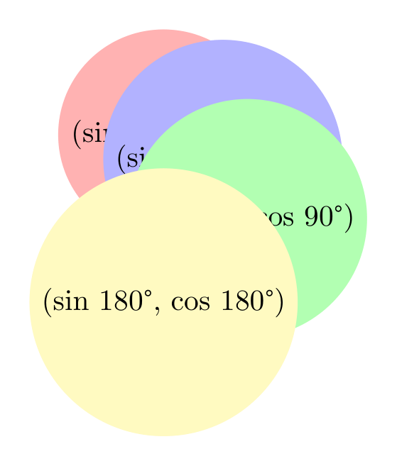
Show Tikz code
print(fig)% --------------------------------------------- %% Tikzfigure generated by tikzfigure v0.3.1 %% https://github.com/max-models/tikzfigure %% --------------------------------------------- %\begin{tikzpicture} \node[shape=circle, fill=red!30] (P0) at ({sin(0)}, {cos(0)}) {(sin 0°, cos 0°)}; \node[shape=circle, fill=blue!30] (P45) at ({sin(45)}, {cos(45)}) {(sin 45°, cos 45°)}; \node[shape=circle, fill=green!30] (P90) at ({sin(90)}, {cos(90)}) {(sin 90°, cos 90°)}; \node[shape=circle, fill=yellow!30] (P180) at ({sin(180)}, {cos(180)}) {(sin 180°, cos 180°)}; \draw[->, color=gray, line width=1.5] (sin(0), cos(0)) to (sin(45), cos(45)) to (sin(90), cos(90)) to (sin(180), cos(180));\end{tikzpicture}print(fig.generate_standalone())\documentclass[border=10pt]{standalone}\PassOptionsToPackage{dvipsnames,svgnames,x11names}{xcolor}\usepackage{tikz}\usepackage{pgfplots}\pgfplotsset{compat=newest}\usepgfplotslibrary{groupplots}\usetikzlibrary{arrows.meta}\begin{document}% --------------------------------------------- %% Tikzfigure generated by tikzfigure v0.3.1 %% https://github.com/max-models/tikzfigure %% --------------------------------------------- %\begin{tikzpicture} \node[shape=circle, fill=red!30] (P0) at ({sin(0)}, {cos(0)}) {(sin 0°, cos 0°)}; \node[shape=circle, fill=blue!30] (P45) at ({sin(45)}, {cos(45)}) {(sin 45°, cos 45°)}; \node[shape=circle, fill=green!30] (P90) at ({sin(90)}, {cos(90)}) {(sin 90°, cos 90°)}; \node[shape=circle, fill=yellow!30] (P180) at ({sin(180)}, {cos(180)}) {(sin 180°, cos 180°)}; \draw[->, color=gray, line width=1.5] (sin(0), cos(0)) to (sin(45), cos(45)) to (sin(90), cos(90)) to (sin(180), cos(180));\end{tikzpicture}
\end{document}Operators and composition
Section titled “Operators and composition”Expressions support Python’s arithmetic operators (+, -, *, /)
and exponentiation (**). The operators are translated to valid PGF
syntax:
# Build complex expressions using operatorsexpr_sum = sin(60) + cos(60)expr_product = sin(60) * 2expr_power = sin(45) ** 2  # Note: ** becomes ^ in PGFexpr_composed = (sin(45) ** 2 + cos(45) ** 2) / Var("scale")
print(f"sin(60) + cos(60) = {expr_sum}")print(f"sin(60) * 2 = {expr_product}")print(f"sin(45) ** 2 = {expr_power}")print(    f"(sin(45)^2 + cos(45)^2) / scale = {expr_composed}",)
sin(60) + cos(60) = (sin(60) + cos(60))sin(60) * 2 = (sin(60) * 2)sin(45) ** 2 = (sin(45)^2)(sin(45)^2 + cos(45)^2) / scale = (((sin(45)^2) + (cos(45)^2)) / \scale)Variable references with Var()
Section titled “Variable references with Var()”Use Var(name) to reference a PGF variable by name. This is useful when
you define variables with variable() and want to use them in
expressions:
fig = TikzFigure()
# Define a variablefig.variable("radius", 3.5)
# Use it in node coordinatesnode_a = fig.node(    (Var("radius"), 0),    label="A",    content="(r, 0)",    fill="blue!30",    shape="circle",)node_b = fig.node(    (0, Var("radius")),    label="B",    content="(0, r)",    fill="red!30",    shape="circle",)
# Draw using the variablefig.draw(    [(Var("radius"), 0), (0, Var("radius"))],    arrows=arrows.forward,    color="gray",)
fig.show()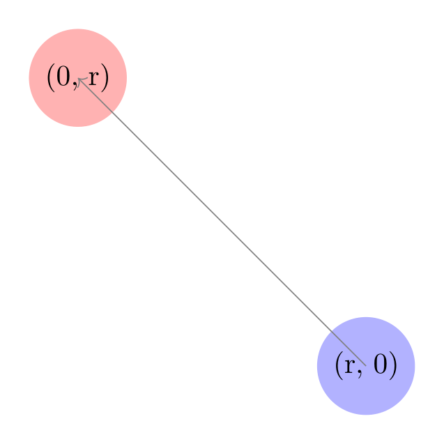
Show Tikz code
print(fig)% --------------------------------------------- %% Tikzfigure generated by tikzfigure v0.3.1 %% https://github.com/max-models/tikzfigure %% --------------------------------------------- %\begin{tikzpicture} \pgfmathsetmacro{\radius}{3.5} \node[shape=circle, fill=blue!30] (A) at ({\radius}, {0}) {(r, 0)}; \node[shape=circle, fill=red!30] (B) at ({0}, {\radius}) {(0, r)}; \draw[->, color=gray] (\radius, 0) to (0, \radius);\end{tikzpicture}print(fig.generate_standalone())\documentclass[border=10pt]{standalone}\PassOptionsToPackage{dvipsnames,svgnames,x11names}{xcolor}\usepackage{tikz}\usepackage{pgfplots}\pgfplotsset{compat=newest}\usepgfplotslibrary{groupplots}\usetikzlibrary{arrows.meta}\begin{document}% --------------------------------------------- %% Tikzfigure generated by tikzfigure v0.3.1 %% https://github.com/max-models/tikzfigure %% --------------------------------------------- %\begin{tikzpicture} \pgfmathsetmacro{\radius}{3.5} \node[shape=circle, fill=blue!30] (A) at ({\radius}, {0}) {(r, 0)}; \node[shape=circle, fill=red!30] (B) at ({0}, {\radius}) {(0, r)}; \draw[->, color=gray] (\radius, 0) to (0, \radius);\end{tikzpicture}
\end{document}Expressions in variables
Section titled “Expressions in variables”You can pass expressions directly to variable(). This is powerful for
defining derived or computed values at compile time:
fig = TikzFigure()
# Define base variables (coordinates of a point)fig.variable("x", 3)fig.variable("y", 4)
# Compute distance from origin and anglefig.variable(    "distance",    sqrt(Var("x") ** 2 + Var("y") ** 2),)fig.variable("angle", "atan2(\\y, \\x)")  # PGF math: angle in radiansfig.variable("scaled", Var("distance") * 2)
# Place nodes at (x, y), (distance, 0), and (scaled, 0)fig.node(    (Var("x"), Var("y")),    label="(x, y)",    content="(x, y)",    fill="blue!20",    shape="circle",)fig.node(    (Var("distance"), 0),    label="distance",    content="distance",    fill="green!30",    shape="circle",)fig.node(    (Var("scaled"), 0),    label="scaled",    content="scaled",    fill="purple!30",    shape="circle",)
# Draw a line from origin to (x, y)fig.draw(    [(0, 0), (Var("x"), Var("y"))],    arrows=arrows.forward,    color="gray",)
fig.show()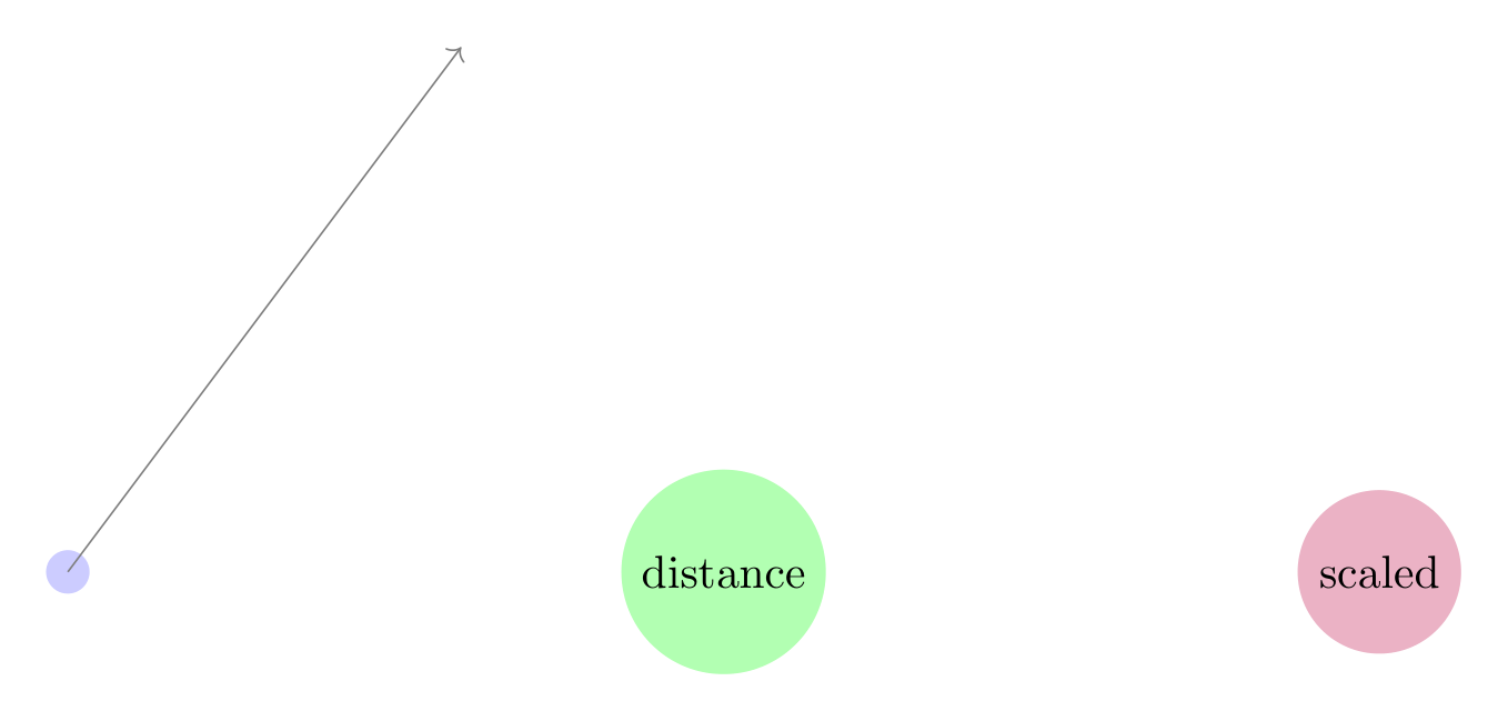
Show Tikz code
print(fig)% --------------------------------------------- %% Tikzfigure generated by tikzfigure v0.3.1 %% https://github.com/max-models/tikzfigure %% --------------------------------------------- %\begin{tikzpicture} \pgfmathsetmacro{\x}{3} \pgfmathsetmacro{\y}{4} \pgfmathsetmacro{\distance}{sqrt(((\x^2) + (\y^2)))} \pgfmathsetmacro{\angle}{atan2(\y, \x)} \pgfmathsetmacro{\scaled}{(\distance * 2)} \node[shape=circle, fill=blue!20] ((x, y)) at ({\x}, {\y}) {(x, y)}; \node[shape=circle, fill=green!30] (distance) at ({\distance}, {0}) {distance}; \node[shape=circle, fill=purple!30] (scaled) at ({\scaled}, {0}) {scaled}; \draw[->, color=gray] (0, 0) to (\x, \y);\end{tikzpicture}print(fig.generate_standalone())\documentclass[border=10pt]{standalone}\PassOptionsToPackage{dvipsnames,svgnames,x11names}{xcolor}\usepackage{tikz}\usepackage{pgfplots}\pgfplotsset{compat=newest}\usepgfplotslibrary{groupplots}\usetikzlibrary{arrows.meta}\begin{document}% --------------------------------------------- %% Tikzfigure generated by tikzfigure v0.3.1 %% https://github.com/max-models/tikzfigure %% --------------------------------------------- %\begin{tikzpicture} \pgfmathsetmacro{\x}{3} \pgfmathsetmacro{\y}{4} \pgfmathsetmacro{\distance}{sqrt(((\x^2) + (\y^2)))} \pgfmathsetmacro{\angle}{atan2(\y, \x)} \pgfmathsetmacro{\scaled}{(\distance * 2)} \node[shape=circle, fill=blue!20] ((x, y)) at ({\x}, {\y}) {(x, y)}; \node[shape=circle, fill=green!30] (distance) at ({\distance}, {0}) {distance}; \node[shape=circle, fill=purple!30] (scaled) at ({\scaled}, {0}) {scaled}; \draw[->, color=gray] (0, 0) to (\x, \y);\end{tikzpicture}
\end{document}Note: the generated TikZ emits \pgfmathsetmacro commands with the
expression as-is. PGF evaluates these at compile time.
Mathematical functions
Section titled “Mathematical functions”The math module includes 60+ PGF functions:
Trigonometric: sin, cos, tan, asin, acos, atan, atan2,
sec, cosec, cot, sinh, cosh, tanh
Rounding: abs, ceil, floor, round (⚠️ shadows Python
built-ins)
Power & logarithm: sqrt, pow, exp, ln, log2, log10
Min/max: min, max (⚠️ shadows Python built-ins)
Arithmetic: neg, mod, div, frac, gcd, factorial
Logic: and_, or_, not_, iseven, isodd, isprime
Comparison: equal, greater, less, notequal, notgreater,
notless
Geometry: width, height, depth, veclen
Other: deg, rad, int_, real, scalar, bin_, oct_,
hex_, ifthenelse
from tikzfigure.math import (    sin,    cos,    sqrt,    max,    min,  # Common ones    ln,    log10,  # Logarithms    deg,    rad,  # Angle conversion    gcd,    factorial,  # Arithmetic    iseven,    isodd,  # Logic)
# Examplesprint(f"sqrt(2) = {sqrt(2)}")print(f"max(3, 5) = {max(3, 5)}")print(f"ln(e) = {ln('e')}")print(f"deg(pi) = {deg('pi')}")print(f"factorial(5) = {factorial(5)}")print(f"iseven(4) = {iseven(4)}")
sqrt(2) = sqrt(2)max(3, 5) = max(3, 5)ln(e) = ln(e)deg(pi) = deg(pi)factorial(5) = factorial(5)iseven(4) = iseven(4)Constants
Section titled “Constants”Pre-defined constants are available as expressions:
from tikzfigure.math import pi, e, rnd, rand, true, false
print(f"pi = {pi}")print(f"e = {e}")print(f"rnd = {rnd}")  # Random [0, 1)print(f"true = {true}")print(f"false = {false}")
pi = pie = ernd = rndtrue = truefalse = falseA practical example: plotting a circle
Section titled “A practical example: plotting a circle”Here’s a complete example using expressions to parametrically place points around a circle:
from tikzfigure.math import sin, cos, pi, Var
fig = TikzFigure(figsize=(8, 8))
# Define the radius as a variablefig.variable("R", 3)
# Place 12 points around a circle at 30° intervalsnum_points = 12for i in range(num_points):    angle = i * 360 / num_points    x = Var("R") * cos(angle)    y = Var("R") * sin(angle)    fig.node(        (x, y),        label=f"P{i}",        content=str(i),        shape="circle",        fill="blue!40",        minimum_size="0.5cm",    )
# Draw the circle by connecting consecutive pointsfor i in range(num_points):    angle1 = i * 360 / num_points    angle2 = ((i + 1) % num_points) * 360 / num_points
    p1 = (Var("R") * cos(angle1), Var("R") * sin(angle1))    p2 = (Var("R") * cos(angle2), Var("R") * sin(angle2))
    fig.draw(        [p1, p2],        options=["very thin"],        color="gray",    )
# Add a central nodefig.node(    (0, 0),    label="center",    content="C",    shape="circle",    fill="red!40",)
fig.show()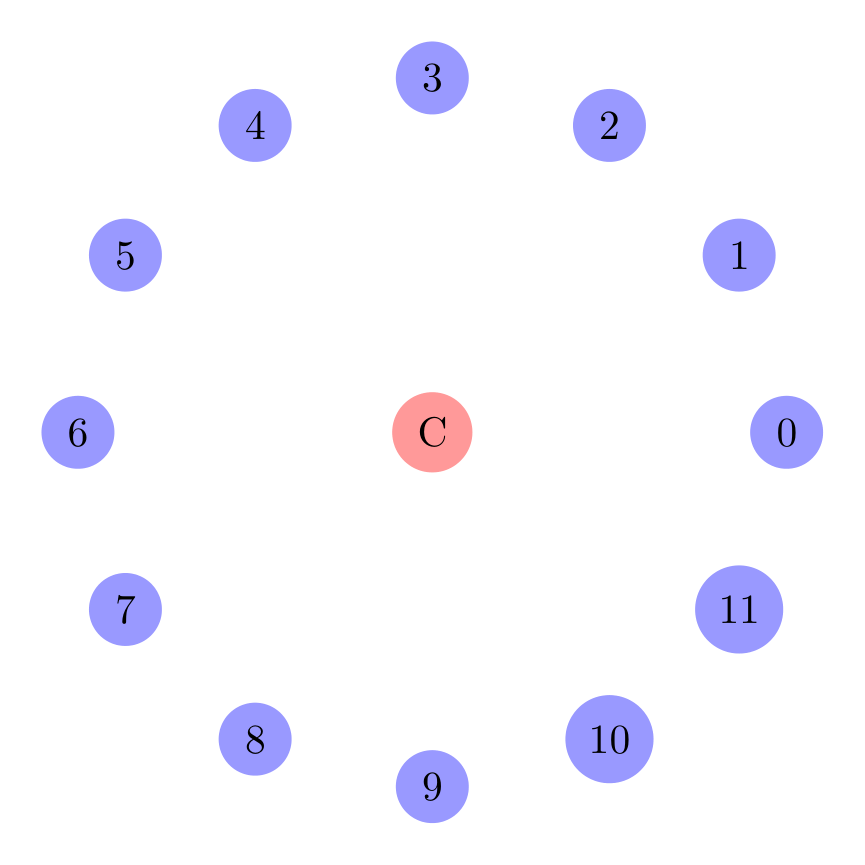
Show Tikz code
print(fig)% --------------------------------------------- %% Tikzfigure generated by tikzfigure v0.3.1 %% https://github.com/max-models/tikzfigure %% --------------------------------------------- %\begin{tikzpicture} \pgfmathsetmacro{\R}{3} \node[shape=circle, fill=blue!40, minimum size=0.5cm] (P0) at ({\R * cos(0.0)}, {\R * sin(0.0)}) {0}; \node[shape=circle, fill=blue!40, minimum size=0.5cm] (P1) at ({\R * cos(30.0)}, {\R * sin(30.0)}) {1}; \node[shape=circle, fill=blue!40, minimum size=0.5cm] (P2) at ({\R * cos(60.0)}, {\R * sin(60.0)}) {2}; \node[shape=circle, fill=blue!40, minimum size=0.5cm] (P3) at ({\R * cos(90.0)}, {\R * sin(90.0)}) {3}; \node[shape=circle, fill=blue!40, minimum size=0.5cm] (P4) at ({\R * cos(120.0)}, {\R * sin(120.0)}) {4}; \node[shape=circle, fill=blue!40, minimum size=0.5cm] (P5) at ({\R * cos(150.0)}, {\R * sin(150.0)}) {5}; \node[shape=circle, fill=blue!40, minimum size=0.5cm] (P6) at ({\R * cos(180.0)}, {\R * sin(180.0)}) {6}; \node[shape=circle, fill=blue!40, minimum size=0.5cm] (P7) at ({\R * cos(210.0)}, {\R * sin(210.0)}) {7}; \node[shape=circle, fill=blue!40, minimum size=0.5cm] (P8) at ({\R * cos(240.0)}, {\R * sin(240.0)}) {8}; \node[shape=circle, fill=blue!40, minimum size=0.5cm] (P9) at ({\R * cos(270.0)}, {\R * sin(270.0)}) {9}; \node[shape=circle, fill=blue!40, minimum size=0.5cm] (P10) at ({\R * cos(300.0)}, {\R * sin(300.0)}) {10}; \node[shape=circle, fill=blue!40, minimum size=0.5cm] (P11) at ({\R * cos(330.0)}, {\R * sin(330.0)}) {11}; \draw[very thin, color=gray] (\R * cos(0.0), \R * sin(0.0)) to (\R * cos(30.0), \R * sin(30.0)); \draw[very thin, color=gray] (\R * cos(30.0), \R * sin(30.0)) to (\R * cos(60.0), \R * sin(60.0)); \draw[very thin, color=gray] (\R * cos(60.0), \R * sin(60.0)) to (\R * cos(90.0), \R * sin(90.0)); \draw[very thin, color=gray] (\R * cos(90.0), \R * sin(90.0)) to (\R * cos(120.0), \R * sin(120.0)); \draw[very thin, color=gray] (\R * cos(120.0), \R * sin(120.0)) to (\R * cos(150.0), \R * sin(150.0)); \draw[very thin, color=gray] (\R * cos(150.0), \R * sin(150.0)) to (\R * cos(180.0), \R * sin(180.0)); \draw[very thin, color=gray] (\R * cos(180.0), \R * sin(180.0)) to (\R * cos(210.0), \R * sin(210.0)); \draw[very thin, color=gray] (\R * cos(210.0), \R * sin(210.0)) to (\R * cos(240.0), \R * sin(240.0)); \draw[very thin, color=gray] (\R * cos(240.0), \R * sin(240.0)) to (\R * cos(270.0), \R * sin(270.0)); \draw[very thin, color=gray] (\R * cos(270.0), \R * sin(270.0)) to (\R * cos(300.0), \R * sin(300.0)); \draw[very thin, color=gray] (\R * cos(300.0), \R * sin(300.0)) to (\R * cos(330.0), \R * sin(330.0)); \draw[very thin, color=gray] (\R * cos(330.0), \R * sin(330.0)) to (\R * cos(0.0), \R * sin(0.0)); \node[shape=circle, fill=red!40] (center) at ({0}, {0}) {C};\end{tikzpicture}print(fig.generate_standalone())\documentclass[border=10pt]{standalone}\PassOptionsToPackage{dvipsnames,svgnames,x11names}{xcolor}\usepackage{tikz}\usepackage{pgfplots}\pgfplotsset{compat=newest}\usepgfplotslibrary{groupplots}\usetikzlibrary{arrows.meta}\begin{document}% --------------------------------------------- %% Tikzfigure generated by tikzfigure v0.3.1 %% https://github.com/max-models/tikzfigure %% --------------------------------------------- %\begin{tikzpicture} \pgfmathsetmacro{\R}{3} \node[shape=circle, fill=blue!40, minimum size=0.5cm] (P0) at ({\R * cos(0.0)}, {\R * sin(0.0)}) {0}; \node[shape=circle, fill=blue!40, minimum size=0.5cm] (P1) at ({\R * cos(30.0)}, {\R * sin(30.0)}) {1}; \node[shape=circle, fill=blue!40, minimum size=0.5cm] (P2) at ({\R * cos(60.0)}, {\R * sin(60.0)}) {2}; \node[shape=circle, fill=blue!40, minimum size=0.5cm] (P3) at ({\R * cos(90.0)}, {\R * sin(90.0)}) {3}; \node[shape=circle, fill=blue!40, minimum size=0.5cm] (P4) at ({\R * cos(120.0)}, {\R * sin(120.0)}) {4}; \node[shape=circle, fill=blue!40, minimum size=0.5cm] (P5) at ({\R * cos(150.0)}, {\R * sin(150.0)}) {5}; \node[shape=circle, fill=blue!40, minimum size=0.5cm] (P6) at ({\R * cos(180.0)}, {\R * sin(180.0)}) {6}; \node[shape=circle, fill=blue!40, minimum size=0.5cm] (P7) at ({\R * cos(210.0)}, {\R * sin(210.0)}) {7}; \node[shape=circle, fill=blue!40, minimum size=0.5cm] (P8) at ({\R * cos(240.0)}, {\R * sin(240.0)}) {8}; \node[shape=circle, fill=blue!40, minimum size=0.5cm] (P9) at ({\R * cos(270.0)}, {\R * sin(270.0)}) {9}; \node[shape=circle, fill=blue!40, minimum size=0.5cm] (P10) at ({\R * cos(300.0)}, {\R * sin(300.0)}) {10}; \node[shape=circle, fill=blue!40, minimum size=0.5cm] (P11) at ({\R * cos(330.0)}, {\R * sin(330.0)}) {11}; \draw[very thin, color=gray] (\R * cos(0.0), \R * sin(0.0)) to (\R * cos(30.0), \R * sin(30.0)); \draw[very thin, color=gray] (\R * cos(30.0), \R * sin(30.0)) to (\R * cos(60.0), \R * sin(60.0)); \draw[very thin, color=gray] (\R * cos(60.0), \R * sin(60.0)) to (\R * cos(90.0), \R * sin(90.0)); \draw[very thin, color=gray] (\R * cos(90.0), \R * sin(90.0)) to (\R * cos(120.0), \R * sin(120.0)); \draw[very thin, color=gray] (\R * cos(120.0), \R * sin(120.0)) to (\R * cos(150.0), \R * sin(150.0)); \draw[very thin, color=gray] (\R * cos(150.0), \R * sin(150.0)) to (\R * cos(180.0), \R * sin(180.0)); \draw[very thin, color=gray] (\R * cos(180.0), \R * sin(180.0)) to (\R * cos(210.0), \R * sin(210.0)); \draw[very thin, color=gray] (\R * cos(210.0), \R * sin(210.0)) to (\R * cos(240.0), \R * sin(240.0)); \draw[very thin, color=gray] (\R * cos(240.0), \R * sin(240.0)) to (\R * cos(270.0), \R * sin(270.0)); \draw[very thin, color=gray] (\R * cos(270.0), \R * sin(270.0)) to (\R * cos(300.0), \R * sin(300.0)); \draw[very thin, color=gray] (\R * cos(300.0), \R * sin(300.0)) to (\R * cos(330.0), \R * sin(330.0)); \draw[very thin, color=gray] (\R * cos(330.0), \R * sin(330.0)) to (\R * cos(0.0), \R * sin(0.0)); \node[shape=circle, fill=red!40] (center) at ({0}, {0}) {C};\end{tikzpicture}
\end{document}The expressions are evaluated by PGF at compile time, not Python, so the generated LaTeX is clean and readable — not a long list of hardcoded coordinates.
Advanced: combining loops with expressions
Section titled “Advanced: combining loops with expressions”For parametric figures like grids or circles, you can combine TikZ
\foreach loops (from tutorial 6) with math
expressions for even more compact code:
from tikzfigure.math import sin, cos, Var
fig = TikzFigure(figsize=(8, 8))
# Define radiusfig.variable("R", 2.5)
# Use TikZ \foreach loop with math expressionswith fig.loop(    "i",    range(8),    comment="Circle with 8 points",) as loop:    # Position: (R * cos(i*45°), R * sin(i*45°))    x = Var("R") * cos(r"\i * 45")    y = Var("R") * sin(r"\i * 45")
    loop.node(        (x, y),        label=r"P\i",        content=r"\i",        shape="circle",        fill="blue!40",        minimum_size="0.6cm",    )
# Add centerfig.node(    (0, 0),    label="O",    content="O",    shape="circle",    fill="red!30",)fig.show()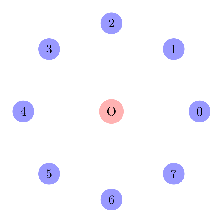
Show Tikz code
print(fig)% --------------------------------------------- %% Tikzfigure generated by tikzfigure v0.3.1 %% https://github.com/max-models/tikzfigure %% --------------------------------------------- %\begin{tikzpicture} \pgfmathsetmacro{\R}{2.5} % Circle with 8 points \foreach \i in {0,1,...,7}{ \node[shape=circle, fill=blue!40, minimum size=0.6cm] (P\i) at ({\R * cos(\i * 45)}, {\R * sin(\i * 45)}) {\i}; } \node[shape=circle, fill=red!30] (O) at ({0}, {0}) {O};\end{tikzpicture}print(fig.generate_standalone())\documentclass[border=10pt]{standalone}\PassOptionsToPackage{dvipsnames,svgnames,x11names}{xcolor}\usepackage{tikz}\usepackage{pgfplots}\pgfplotsset{compat=newest}\usepgfplotslibrary{groupplots}\usetikzlibrary{arrows.meta}\begin{document}% --------------------------------------------- %% Tikzfigure generated by tikzfigure v0.3.1 %% https://github.com/max-models/tikzfigure %% --------------------------------------------- %\begin{tikzpicture} \pgfmathsetmacro{\R}{2.5} % Circle with 8 points \foreach \i in {0,1,...,7}{ \node[shape=circle, fill=blue!40, minimum size=0.6cm] (P\i) at ({\R * cos(\i * 45)}, {\R * sin(\i * 45)}) {\i}; } \node[shape=circle, fill=red!30] (O) at ({0}, {0}) {O};\end{tikzpicture}
\end{document}Notice how the loop variable \i is embedded in the math expressions.
TikZ evaluates \i * 45 at each iteration, then passes it to cos()
and sin().
Next step: parametric TikZ plots
Section titled “Next step: parametric TikZ plots”If you want to go further and use declared PGF functions together with
plain TikZ plot(...) commands, continue with Tokamak X-Point with
Parametric TikZ Plots. That
tutorial starts with a single simple sampled curve and builds up step by
step to a stylized tokamak separatrix / X-point drawing.
Warning: shadowing Python built-ins
Section titled “Warning: shadowing Python built-ins”Some PGF functions have names that match Python built-ins:
abs,min,max,roundfromtikzfigure.mathshadow Python’s built-ins
This is intentional and fine when using targeted imports:
from tikzfigure.math import sin, cos # No shadowingfrom tikzfigure.math import abs, max # Shadows Python built-ins in this scopeTo avoid confusion, avoid from tikzfigure.math import * (which would
shadow globally).
Next steps
Section titled “Next steps”- Combine expressions with loops for parametric grids
- Use expressions in styling and transformations
- See the PGF manual for the full list of functions and their behavior