Mixed Subfigures: Plots and Diagrams
from tikzfigure import TikzFigure, arrows, stylesMixed Subfigures: Combining Plots and Diagrams
Section titled “Mixed Subfigures: Combining Plots and Diagrams”Create sophisticated figures that combine axis-based plots with custom TikZ diagrams (nodes, paths, shapes). Mix them freely in grid layouts.
Side-by-Side: Plot and Diagram
Section titled “Side-by-Side: Plot and Diagram”The simplest case: an axis-based plot next to a TikZ diagram.
fig = TikzFigure(rows=1, cols=2)
# Left: Axis with plotax = fig.subfigure_axis(    xlabel="x",    ylabel="y",    width=0.5,)ax.add_plot(    [0, 1, 2],    [0, 1, 4],    label="$y=x^2$",    marker="o",)ax.set_legend()
# Right: TikZ diagram with nodes and pathsdiagram = fig.subfigure(width=0.5)A = diagram.node(    0,    2,    label="A",    content="A",    shape="circle",    fill="cyan!40",)B = diagram.node(    3,    2,    label="B",    content="B",    shape="circle",    fill="cyan!40",)C = diagram.node(    0,    0,    label="C",    content="C",    shape="circle",    fill="cyan!40",)D = diagram.node(    3,    0,    label="D",    content="D",    shape="circle",    fill="cyan!40",)diagram.draw([A, B], arrows=arrows.forward)diagram.draw([A, C], arrows=arrows.forward)diagram.draw([B, D], arrows=arrows.forward)diagram.draw([C, D], arrows=arrows.forward)diagram.draw(    [A, D],    arrows=arrows.forward,    options=[styles.dashed],    bend_left=20,    color="gray",)
fig.show()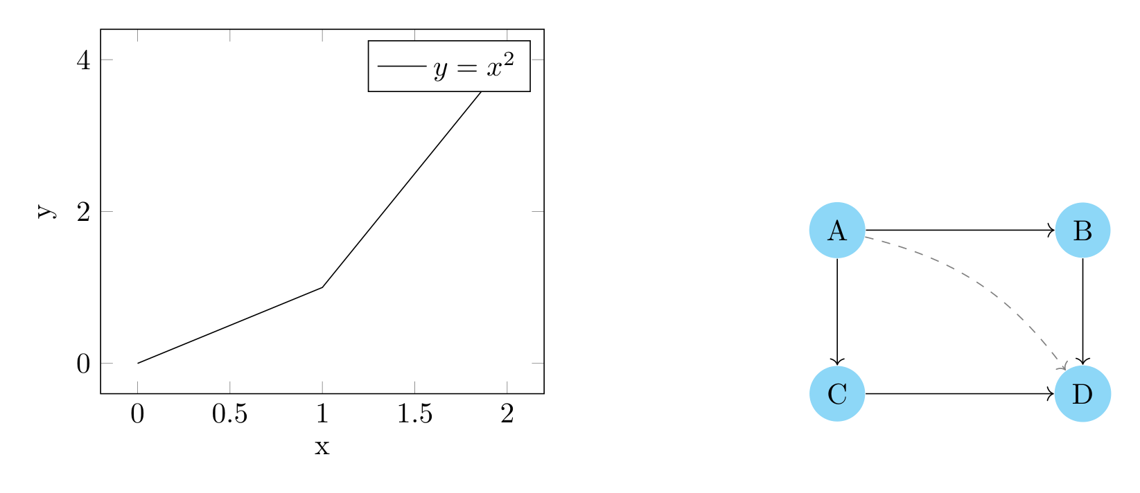
Show Tikz code
print(fig)\begin{tikzpicture} \begin{scope}[xshift=0.0cm, yshift=0.0cm] \begin{axis}[width=7.0cm, xlabel=x, ylabel=y, grid=major, legend pos=north east] \addplot[marker=o] coordinates {(0,0) (1,1) (2,4)}; \legend{$y=x^2$} \end{axis} \end{scope} \begin{scope}[xshift=8.5cm, yshift=0.0cm] \node[shape=circle, fill=cyan!40] (A) at ({0}, {2}) {A}; \node[shape=circle, fill=cyan!40] (B) at ({3}, {2}) {B}; \node[shape=circle, fill=cyan!40] (C) at ({0}, {0}) {C}; \node[shape=circle, fill=cyan!40] (D) at ({3}, {0}) {D}; \draw[->] (A) to (B); \draw[->] (A) to (C); \draw[->] (B) to (D); \draw[->] (C) to (D); \draw[dashed, ->, color=gray, bend left=20] (A) to (D); \end{scope}\end{tikzpicture}print(fig.generate_standalone())\documentclass[border=10pt]{standalone}\PassOptionsToPackage{dvipsnames,svgnames,x11names}{xcolor}\usepackage{tikz}\usepackage{pgfplots}\pgfplotsset{compat=newest}\usepgfplotslibrary{groupplots}\usetikzlibrary{arrows.meta}\begin{document}\begin{tikzpicture} \begin{scope}[xshift=0.0cm, yshift=0.0cm] \begin{axis}[width=7.0cm, xlabel=x, ylabel=y, grid=major, legend pos=north east] \addplot[marker=o] coordinates {(0,0) (1,1) (2,4)}; \legend{$y=x^2$} \end{axis} \end{scope} \begin{scope}[xshift=8.5cm, yshift=0.0cm] \node[shape=circle, fill=cyan!40] (A) at ({0}, {2}) {A}; \node[shape=circle, fill=cyan!40] (B) at ({3}, {2}) {B}; \node[shape=circle, fill=cyan!40] (C) at ({0}, {0}) {C}; \node[shape=circle, fill=cyan!40] (D) at ({3}, {0}) {D}; \draw[->] (A) to (B); \draw[->] (A) to (C); \draw[->] (B) to (D); \draw[->] (C) to (D); \draw[dashed, ->, color=gray, bend left=20] (A) to (D); \end{scope}\end{tikzpicture}
\end{document}Key API: - fig.subfigure_axis() — Create an axis-based subplot -
fig.subfigure() — Create a bare TikZ diagram subplot - Both return
objects you can populate with plots or drawings
2×2 Grid: Mix Freely
Section titled “2×2 Grid: Mix Freely”Create a 2×2 grid with plots and diagrams in any arrangement.
fig = TikzFigure(rows=2, cols=2)
# Top-left: Linear plotax1 = fig.subfigure_axis(    xlabel="x",    ylabel="y",    width=0.45,)ax1.add_plot(    [0, 1, 2, 3],    [0, 1, 2, 3],    label="Linear",    marker="o",)ax1.set_legend()
# Top-right: Quadratic plotax2 = fig.subfigure_axis(    xlabel="x",    ylabel="y",    width=0.45,)ax2.add_plot(    [0, 1, 2, 3],    [0, 1, 4, 9],    label="Quadratic",    marker="s",)ax2.set_legend()
# Bottom-left: Diagram - simple flowchartflowchart = fig.subfigure(width=0.45, height=5)start = flowchart.node(    1.5,    3,    label="start",    content="Start",    shape="circle",    fill="green!40",)process = flowchart.node(    1.5,    1.5,    label="process",    content="Process",    shape="rectangle",    fill="yellow!40",)end = flowchart.node(    1.5,    0,    label="end",    content="End",    shape="circle",    fill="red!40",)flowchart.draw([start, process], arrows=arrows.forward)flowchart.draw([process, end], arrows=arrows.forward)
# Bottom-right: Diagram - networknetwork = fig.subfigure(width=0.45, height=5)center = network.node(    1.5,    1.5,    label="center",    content="Hub",    shape="circle",    fill="purple!40",    minimum_size="15pt",)n1 = network.node(    0.5,    2.5,    label="n1",    content="Node 1",    shape="circle",    fill="cyan!40",)n2 = network.node(    2.5,    2.5,    label="n2",    content="Node 2",    shape="circle",    fill="cyan!40",)n3 = network.node(    0.5,    0.5,    label="n3",    content="Node 3",    shape="circle",    fill="cyan!40",)n4 = network.node(    2.5,    0.5,    label="n4",    content="Node 4",    shape="circle",    fill="cyan!40",)network.draw([center, n1], options=[styles.thick])network.draw([center, n2], options=[styles.thick])network.draw([center, n3], options=[styles.thick])network.draw([center, n4], options=[styles.thick])
fig.show()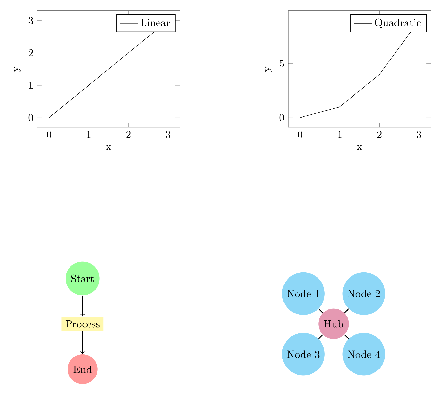
Show Tikz code
print(fig)\begin{tikzpicture} \begin{scope}[xshift=0.0cm, yshift=0.0cm] \begin{axis}[width=6.3cm, xlabel=x, ylabel=y, grid=major, legend pos=north east] \addplot[marker=o] coordinates {(0,0) (1,1) (2,2) (3,3)}; \legend{Linear} \end{axis} \end{scope} \begin{scope}[xshift=7.8cm, yshift=0.0cm] \begin{axis}[width=6.3cm, xlabel=x, ylabel=y, grid=major, legend pos=north east] \addplot[marker=s] coordinates {(0,0) (1,1) (2,4) (3,9)}; \legend{Quadratic} \end{axis} \end{scope} \begin{scope}[xshift=0.0cm, yshift=-8.0cm] \node[shape=circle, fill=green!40] (start) at ({1.5}, {3}) {Start}; \node[shape=rectangle, fill=yellow!40] (process) at ({1.5}, {1.5}) {Process}; \node[shape=circle, fill=red!40] (end) at ({1.5}, {0}) {End}; \draw[->] (start) to (process); \draw[->] (process) to (end); \end{scope} \begin{scope}[xshift=7.8cm, yshift=-8.0cm] \node[shape=circle, fill=purple!40, minimum size=15pt] (center) at ({1.5}, {1.5}) {Hub}; \node[shape=circle, fill=cyan!40] (n1) at ({0.5}, {2.5}) {Node 1}; \node[shape=circle, fill=cyan!40] (n2) at ({2.5}, {2.5}) {Node 2}; \node[shape=circle, fill=cyan!40] (n3) at ({0.5}, {0.5}) {Node 3}; \node[shape=circle, fill=cyan!40] (n4) at ({2.5}, {0.5}) {Node 4}; \draw[thick] (center) to (n1); \draw[thick] (center) to (n2); \draw[thick] (center) to (n3); \draw[thick] (center) to (n4); \end{scope}\end{tikzpicture}print(fig.generate_standalone())\documentclass[border=10pt]{standalone}\PassOptionsToPackage{dvipsnames,svgnames,x11names}{xcolor}\usepackage{tikz}\usepackage{pgfplots}\pgfplotsset{compat=newest}\usepgfplotslibrary{groupplots}\usetikzlibrary{arrows.meta}\begin{document}\begin{tikzpicture} \begin{scope}[xshift=0.0cm, yshift=0.0cm] \begin{axis}[width=6.3cm, xlabel=x, ylabel=y, grid=major, legend pos=north east] \addplot[marker=o] coordinates {(0,0) (1,1) (2,2) (3,3)}; \legend{Linear} \end{axis} \end{scope} \begin{scope}[xshift=7.8cm, yshift=0.0cm] \begin{axis}[width=6.3cm, xlabel=x, ylabel=y, grid=major, legend pos=north east] \addplot[marker=s] coordinates {(0,0) (1,1) (2,4) (3,9)}; \legend{Quadratic} \end{axis} \end{scope} \begin{scope}[xshift=0.0cm, yshift=-8.0cm] \node[shape=circle, fill=green!40] (start) at ({1.5}, {3}) {Start}; \node[shape=rectangle, fill=yellow!40] (process) at ({1.5}, {1.5}) {Process}; \node[shape=circle, fill=red!40] (end) at ({1.5}, {0}) {End}; \draw[->] (start) to (process); \draw[->] (process) to (end); \end{scope} \begin{scope}[xshift=7.8cm, yshift=-8.0cm] \node[shape=circle, fill=purple!40, minimum size=15pt] (center) at ({1.5}, {1.5}) {Hub}; \node[shape=circle, fill=cyan!40] (n1) at ({0.5}, {2.5}) {Node 1}; \node[shape=circle, fill=cyan!40] (n2) at ({2.5}, {2.5}) {Node 2}; \node[shape=circle, fill=cyan!40] (n3) at ({0.5}, {0.5}) {Node 3}; \node[shape=circle, fill=cyan!40] (n4) at ({2.5}, {0.5}) {Node 4}; \draw[thick] (center) to (n1); \draw[thick] (center) to (n2); \draw[thick] (center) to (n3); \draw[thick] (center) to (n4); \end{scope}\end{tikzpicture}
\end{document}Flowchart with Data Comparison
Section titled “Flowchart with Data Comparison”Combine an algorithm flowchart with performance data.
fig = TikzFigure(rows=2, cols=1)
# Top: Convergence comparisonax = fig.subfigure_axis(    xlabel="Iteration",    ylabel="Error",    width=0.9,)x = [0, 1, 2, 3, 4, 5]ax.add_plot(    x,    [1.0, 0.5, 0.25, 0.125, 0.06, 0.03],    label="Fast",    marker="o",)ax.add_plot(    x,    [1.0, 0.9, 0.8, 0.7, 0.6, 0.5],    label="Slow",    marker="s",)ax.set_legend()
# Bottom: Algorithm flowchartflowchart = fig.subfigure(width=0.9, height=7)
# Build flowchart nodesstart = flowchart.node(    2,    4.5,    label="start",    content="Initialize",    shape="circle",    fill="green!40",)input_node = flowchart.node(    2,    3.5,    label="input",    content="Set Parameters",    shape="rectangle",    fill="cyan!40",)check_iter = flowchart.node(    2,    2.5,    label="check_iter",    content="Iterations < Max?",    shape="diamond",)compute = flowchart.node(    4,    2.5,    label="compute",    content="Compute Step",    shape="rectangle",    fill="yellow!40",)check_conv = flowchart.node(    4,    1.5,    label="check_conv",    content="Converged?",    shape="diamond",)output = flowchart.node(    2,    0.5,    label="output",    content="Output Result",    shape="rectangle",    fill="cyan!40",)end = flowchart.node(    2,    -0.5,    label="end",    content="End",    shape="circle",    fill="red!40",)
# Draw pathsflowchart.draw([start, input_node], arrows=arrows.forward)flowchart.draw(    [input_node, check_iter],    arrows=arrows.forward,)flowchart.draw(    [check_iter, compute],    arrows=arrows.forward,    label="yes",)flowchart.draw([compute, check_conv], arrows=arrows.forward)flowchart.draw(    [check_iter, output],    arrows=arrows.forward,    label="no",)flowchart.draw(    [check_conv, compute],    arrows=arrows.forward,    label="no",    bend_left=30,)flowchart.draw(    [check_conv, output],    arrows=arrows.forward,    label="yes",)flowchart.draw([output, end], arrows=arrows.forward)
fig.show()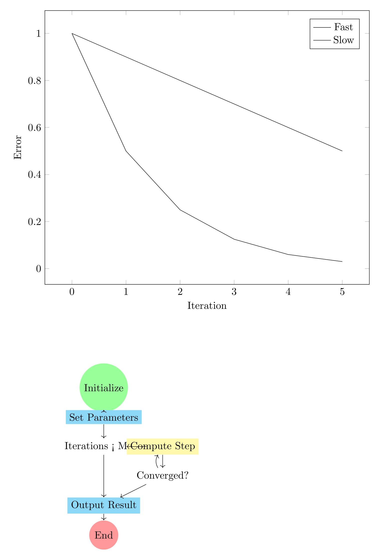
Show Tikz code
print(fig)\begin{tikzpicture} \begin{scope}[xshift=0.0cm, yshift=0.0cm] \begin{axis}[width=12.6cm, xlabel=Iteration, ylabel=Error, grid=major, legend pos=north east] \addplot[marker=o] coordinates {(0,1.0) (1,0.5) (2,0.25) (3,0.125) (4,0.06) (5,0.03)}; \addplot[marker=s] coordinates {(0,1.0) (1,0.9) (2,0.8) (3,0.7) (4,0.6) (5,0.5)}; \legend{Fast, Slow} \end{axis} \end{scope} \begin{scope}[xshift=0.0cm, yshift=-8.0cm] \node[shape=circle, fill=green!40] (start) at ({2}, {4.5}) {Initialize}; \node[shape=rectangle, fill=cyan!40] (input) at ({2}, {3.5}) {Set Parameters}; \node[shape=diamond] (check_iter) at ({2}, {2.5}) {Iterations < Max?}; \node[shape=rectangle, fill=yellow!40] (compute) at ({4}, {2.5}) {Compute Step}; \node[shape=diamond] (check_conv) at ({4}, {1.5}) {Converged?}; \node[shape=rectangle, fill=cyan!40] (output) at ({2}, {0.5}) {Output Result}; \node[shape=circle, fill=red!40] (end) at ({2}, {-0.5}) {End}; \draw[->] (start) to (input); \draw[->] (input) to (check_iter); \draw[->] (check_iter) to (compute); \draw[->] (compute) to (check_conv); \draw[->] (check_iter) to (output); \draw[->, bend left=30] (check_conv) to (compute); \draw[->] (check_conv) to (output); \draw[->] (output) to (end); \end{scope}\end{tikzpicture}print(fig.generate_standalone())\documentclass[border=10pt]{standalone}\PassOptionsToPackage{dvipsnames,svgnames,x11names}{xcolor}\usepackage{tikz}\usepackage{pgfplots}\pgfplotsset{compat=newest}\usepgfplotslibrary{groupplots}\usetikzlibrary{arrows.meta}\begin{document}\begin{tikzpicture} \begin{scope}[xshift=0.0cm, yshift=0.0cm] \begin{axis}[width=12.6cm, xlabel=Iteration, ylabel=Error, grid=major, legend pos=north east] \addplot[marker=o] coordinates {(0,1.0) (1,0.5) (2,0.25) (3,0.125) (4,0.06) (5,0.03)}; \addplot[marker=s] coordinates {(0,1.0) (1,0.9) (2,0.8) (3,0.7) (4,0.6) (5,0.5)}; \legend{Fast, Slow} \end{axis} \end{scope} \begin{scope}[xshift=0.0cm, yshift=-8.0cm] \node[shape=circle, fill=green!40] (start) at ({2}, {4.5}) {Initialize}; \node[shape=rectangle, fill=cyan!40] (input) at ({2}, {3.5}) {Set Parameters}; \node[shape=diamond] (check_iter) at ({2}, {2.5}) {Iterations < Max?}; \node[shape=rectangle, fill=yellow!40] (compute) at ({4}, {2.5}) {Compute Step}; \node[shape=diamond] (check_conv) at ({4}, {1.5}) {Converged?}; \node[shape=rectangle, fill=cyan!40] (output) at ({2}, {0.5}) {Output Result}; \node[shape=circle, fill=red!40] (end) at ({2}, {-0.5}) {End}; \draw[->] (start) to (input); \draw[->] (input) to (check_iter); \draw[->] (check_iter) to (compute); \draw[->] (compute) to (check_conv); \draw[->] (check_iter) to (output); \draw[->, bend left=30] (check_conv) to (compute); \draw[->] (check_conv) to (output); \draw[->] (output) to (end); \end{scope}\end{tikzpicture}
\end{document}State Machine Diagram with Benchmark Data
Section titled “State Machine Diagram with Benchmark Data”Show a state machine alongside benchmark timing data.
fig = TikzFigure(figsize=(10, 5), rows=1, cols=2)
# Left: Timing benchmarkax = fig.subfigure_axis(    xlabel="Input Size",    ylabel="Time (ms)",    width=0.5,)sizes = [10, 20, 30, 40, 50]time_state1 = [5, 10, 15, 20, 25]time_state2 = [2, 3, 4, 5, 6]time_state3 = [1, 1.5, 2, 2.5, 3]ax.add_plot(    sizes,    time_state1,    label="State 1",    marker="o",    plot_style="solid",)ax.add_plot(    sizes,    time_state2,    label="State 2",    marker="s",    plot_style="dashed",)ax.add_plot(    sizes,    time_state3,    label="State 3",    marker="^",    plot_style="dotted",)ax.set_legend()
# Right: State machine diagramstates = fig.subfigure(width=0.5, height=6)
# Create state nodess1 = states.node(    0.5,    2,    label="s1",    content="State 1",    shape="circle",    fill="red!40",    minimum_size="12pt",)s2 = states.node(    2,    2,    label="s2",    content="State 2",    shape="circle",    fill="yellow!40",    minimum_size="12pt",)s3 = states.node(    3.5,    2,    label="s3",    content="State 3",    shape="circle",    fill="green!40",    minimum_size="12pt",)
# Draw transitionsstates.draw([s1, s2], arrows=arrows.forward, label="a")states.draw([s2, s3], arrows=arrows.forward, label="b")states.draw(    [s2, s1],    arrows=arrows.forward,    label="c",    bend_left=20,)states.draw(    [s3, s1],    arrows=arrows.forward,    label="d",    bend_left=-20,)states.draw(    [s1, s1],    arrows=arrows.forward,    label="loop",    bend_right=30,    color="blue",)
fig.show()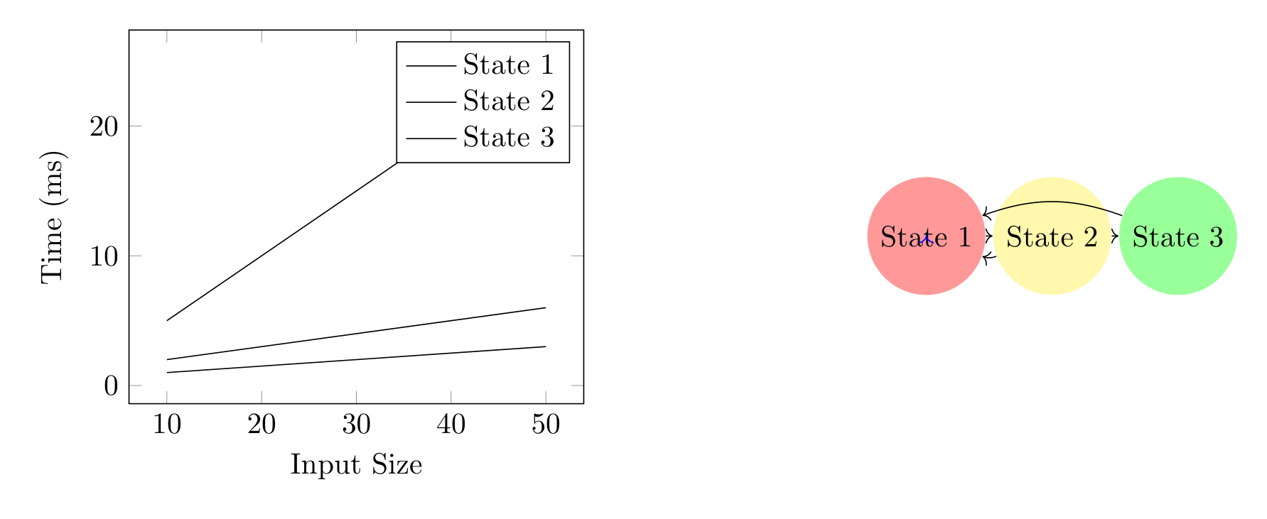
Show Tikz code
print(fig)\begin{tikzpicture} \begin{scope}[xshift=0.0cm, yshift=0.0cm] \begin{axis}[width=7.0cm, xlabel=Input Size, ylabel=Time (ms), grid=major, legend pos=north east] \addplot[marker=o, plot style=solid] coordinates {(10,5) (20,10) (30,15) (40,20) (50,25)}; \addplot[marker=s, plot style=dashed] coordinates {(10,2) (20,3) (30,4) (40,5) (50,6)}; \addplot[marker=^, plot style=dotted] coordinates {(10,1) (20,1.5) (30,2) (40,2.5) (50,3)}; \legend{State 1, State 2, State 3} \end{axis} \end{scope} \begin{scope}[xshift=8.5cm, yshift=0.0cm] \node[shape=circle, fill=red!40, minimum size=12pt] (s1) at ({0.5}, {2}) {State 1}; \node[shape=circle, fill=yellow!40, minimum size=12pt] (s2) at ({2}, {2}) {State 2}; \node[shape=circle, fill=green!40, minimum size=12pt] (s3) at ({3.5}, {2}) {State 3}; \draw[->] (s1) to (s2); \draw[->] (s2) to (s3); \draw[->, bend left=20] (s2) to (s1); \draw[->, bend left=-20] (s3) to (s1); \draw[->, color=blue, bend right=30] (s1) to (s1); \end{scope}\end{tikzpicture}print(fig.generate_standalone())\documentclass[border=10pt]{standalone}\PassOptionsToPackage{dvipsnames,svgnames,x11names}{xcolor}\usepackage{tikz}\usepackage{pgfplots}\pgfplotsset{compat=newest}\usepgfplotslibrary{groupplots}\usetikzlibrary{arrows.meta}\begin{document}\begin{tikzpicture} \begin{scope}[xshift=0.0cm, yshift=0.0cm] \begin{axis}[width=7.0cm, xlabel=Input Size, ylabel=Time (ms), grid=major, legend pos=north east] \addplot[marker=o, plot style=solid] coordinates {(10,5) (20,10) (30,15) (40,20) (50,25)}; \addplot[marker=s, plot style=dashed] coordinates {(10,2) (20,3) (30,4) (40,5) (50,6)}; \addplot[marker=^, plot style=dotted] coordinates {(10,1) (20,1.5) (30,2) (40,2.5) (50,3)}; \legend{State 1, State 2, State 3} \end{axis} \end{scope} \begin{scope}[xshift=8.5cm, yshift=0.0cm] \node[shape=circle, fill=red!40, minimum size=12pt] (s1) at ({0.5}, {2}) {State 1}; \node[shape=circle, fill=yellow!40, minimum size=12pt] (s2) at ({2}, {2}) {State 2}; \node[shape=circle, fill=green!40, minimum size=12pt] (s3) at ({3.5}, {2}) {State 3}; \draw[->] (s1) to (s2); \draw[->] (s2) to (s3); \draw[->, bend left=20] (s2) to (s1); \draw[->, bend left=-20] (s3) to (s1); \draw[->, color=blue, bend right=30] (s1) to (s1); \end{scope}\end{tikzpicture}
\end{document}Tips and Tricks
Section titled “Tips and Tricks”Coordinate Systems: - Both axes and diagrams use their own
coordinate systems - Axes: determined by data (x/y limits) - Diagrams:
you control node positions directly (e.g., node(0, 2, ...) places at
position (0, 2))
Dimensions: - Use height to control vertical space:
subfigure(width=0.45, height=6) - Both axis and diagram subfigures
respect width/height parameters
Styling: - Node fills: fill="cyan!40", fill="red!20", etc. -
Shapes: "circle", "rectangle", "diamond", etc. - Path styling can
use arrows.forward, arrows.both, styles.dashed, styles.thick,
etc. - Bends: bend_left=20, bend_right=30 for curved paths
Mixing in Grids: - Call subfigure_axis() and subfigure() in any
order - They auto-fill left-to-right, top-to-bottom - Both types render
correctly in pgfplots groupplot environment