Coordinates and Midpoints
tikzfigure can compute new node positions geometrically from existing
ones. fig.midpoint(node_a, node_b) places a new node exactly halfway
between two existing nodes. For a lighter alternative with no visible
output, use fig.coordinate(label, x, y) to define a named invisible
waypoint.
This tutorial covers: - basic midpoint usage - point/vector translations
from node positions - using label strings as references - edge labels on
a triangle - recursive bisection - computing a triangle’s centroid via
iterated midpoints - named coordinates as invisible path waypoints -
routing paths via intermediate coordinates - expression-based
coordinates with the calc library
from tikzfigure import TikzFigure, TikzVector, arrows, stylesfig = TikzFigure()
A = fig.node( (0, 0), label="A", content="$A$", shape="circle", fill="blue!20", draw="blue",)B = fig.node( (6, 0), label="B", content="$B$", shape="circle", fill="blue!20", draw="blue",)C = fig.node( (2, 4), label="C", content="$C$", shape="circle", fill="blue!20", draw="blue",)
fig.draw( [A.center, "B", "C"], center=True, cycle=True, color="blue", fill="blue!10", line_width="1.5pt",)
fig.show()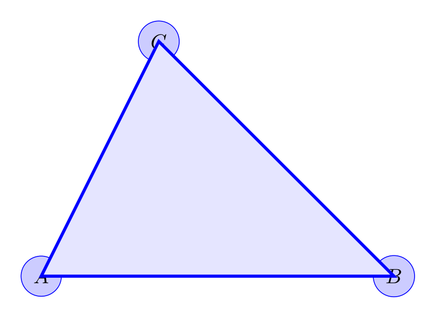
Basic midpoint
Section titled “Basic midpoint”Pass two nodes (or label strings) and any additional node kwargs. The
returned node has .x and .y set to the computed midpoint.
fig = TikzFigure()
n1 = fig.node(    (0, 0),    label="A",    content="A",    shape="circle",    fill="blue!30",    draw="blue",)n2 = fig.node(    (4, 0),    label="B",    content="B",    shape="circle",    fill="red!30",    draw="red",)
mid = fig.midpoint(    n1,    "B",    label="M",    content="M",    shape="circle",    fill="green!30",    draw="green",)
fig.draw([n1, n2], options=[styles.dashed], color="gray")
fig.show()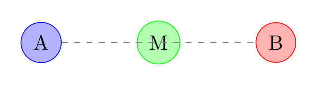
Show Tikz code
print(fig)% --------------------------------------------- %% Tikzfigure generated by tikzfigure v0.3.1 %% https://github.com/max-models/tikzfigure %% --------------------------------------------- %\begin{tikzpicture} \node[shape=circle, fill=blue!30, draw=blue] (A) at ({0}, {0}) {A}; \node[shape=circle, fill=red!30, draw=red] (B) at ({4}, {0}) {B}; \node[shape=circle, fill=green!30, draw=green] (M) at ({2.0}, {0.0}) {M}; \draw[dashed, color=gray] (A) to (B);\end{tikzpicture}print(fig.generate_standalone())\documentclass[border=10pt]{standalone}\PassOptionsToPackage{dvipsnames,svgnames,x11names}{xcolor}\usepackage{tikz}\usepackage{pgfplots}\pgfplotsset{compat=newest}\usepgfplotslibrary{groupplots}\usetikzlibrary{arrows.meta}\begin{document}% --------------------------------------------- %% Tikzfigure generated by tikzfigure v0.3.1 %% https://github.com/max-models/tikzfigure %% --------------------------------------------- %\begin{tikzpicture} \node[shape=circle, fill=blue!30, draw=blue] (A) at ({0}, {0}) {A}; \node[shape=circle, fill=red!30, draw=red] (B) at ({4}, {0}) {B}; \node[shape=circle, fill=green!30, draw=green] (M) at ({2.0}, {0.0}) {M}; \draw[dashed, color=gray] (A) to (B);\end{tikzpicture}
\end{document}Point and vector operations
Section titled “Point and vector operations”Each positioned node exposes its point as node.position. Subtracting
two points gives a TikzVector, and adding a vector to a point
translates it to a new position. That lets you place derived geometry
without retyping coordinates.
fig = TikzFigure()
A = fig.node(    (0, 0),    label="A",    content="$A$",    shape="circle",    fill="blue!20",    draw="blue",)B = fig.node(    (4, 2),    label="B",    content="$B$",    shape="circle",    fill="orange!20",    draw="orange",)
AB = A.vector_to(B)midpoint = A.position + 0.5 * ABoffset = TikzVector(-1, 2)
M = fig.node(    midpoint,    label="M",    content="$M$",    shape="circle",    fill="yellow!40",    draw="yellow!60!black",)A_shifted = fig.node(    A.translate(offset),    label="Ashift",    content="$A+v$",    shape="circle",    fill="green!20",    draw="green!60!black",)
fig.draw([A, B], options=[styles.dashed], color="gray")fig.draw([A, A_shifted], arrows=arrows.forward, color="green!60!black")fig.draw([A, M, B], color="purple")fig.node(    (2, 3.3),    content=rf"$\|AB\| = {A.distance_to(B):.2f}$",    draw="none",)
fig.show()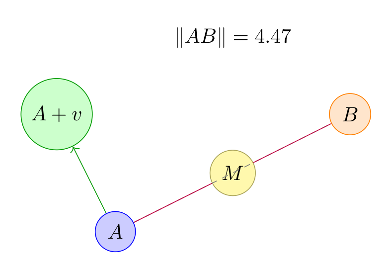
Show Tikz code
print(fig)% --------------------------------------------- %% Tikzfigure generated by tikzfigure v0.3.1 %% https://github.com/max-models/tikzfigure %% --------------------------------------------- %\begin{tikzpicture} \node[shape=circle, fill=blue!20, draw=blue] (A) at ({0}, {0}) {$A$}; \node[shape=circle, fill=orange!20, draw=orange] (B) at ({4}, {2}) {$B$}; \node[shape=circle, fill=yellow!40, draw=yellow!60!black] (M) at ({2.0}, {1.0}) {$M$}; \node[shape=circle, fill=green!20, draw=green!60!black] (Ashift) at ({-1.0}, {2.0}) {$A+v$}; \draw[dashed, color=gray] (A) to (B); \draw[->, color=green!60!black] (A) to (Ashift); \draw[color=purple] (A) to (M) to (B); \node[draw=none] (node4) at ({2}, {3.3}) {$\|AB\| = 4.47$};\end{tikzpicture}print(fig.generate_standalone())\documentclass[border=10pt]{standalone}\PassOptionsToPackage{dvipsnames,svgnames,x11names}{xcolor}\usepackage{tikz}\usepackage{pgfplots}\pgfplotsset{compat=newest}\usepgfplotslibrary{groupplots}\usetikzlibrary{arrows.meta}\begin{document}% --------------------------------------------- %% Tikzfigure generated by tikzfigure v0.3.1 %% https://github.com/max-models/tikzfigure %% --------------------------------------------- %\begin{tikzpicture} \node[shape=circle, fill=blue!20, draw=blue] (A) at ({0}, {0}) {$A$}; \node[shape=circle, fill=orange!20, draw=orange] (B) at ({4}, {2}) {$B$}; \node[shape=circle, fill=yellow!40, draw=yellow!60!black] (M) at ({2.0}, {1.0}) {$M$}; \node[shape=circle, fill=green!20, draw=green!60!black] (Ashift) at ({-1.0}, {2.0}) {$A+v$}; \draw[dashed, color=gray] (A) to (B); \draw[->, color=green!60!black] (A) to (Ashift); \draw[color=purple] (A) to (M) to (B); \node[draw=none] (node4) at ({2}, {3.3}) {$\|AB\| = 4.47$};\end{tikzpicture}
\end{document}Using label strings
Section titled “Using label strings”You can refer to any node by its label string instead of keeping the Python object.
fig = TikzFigure()
fig.node(    (0, 2),    label="P",    content="P",    shape="circle",    fill="orange!40",    draw="orange",)fig.node(    (6, 2),    label="Q",    content="Q",    shape="circle",    fill="orange!40",    draw="orange",)
fig.midpoint(    "P",    "Q",    label="PQ",    content="mid",    shape="circle",    fill="white",    draw="black",)
fig.draw(["P", "Q"], options=[styles.dashed], color="gray")
fig.show()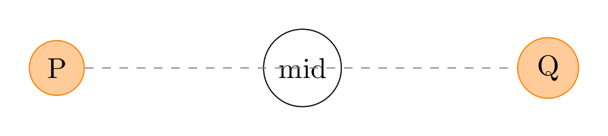
Show Tikz code
print(fig)% --------------------------------------------- %% Tikzfigure generated by tikzfigure v0.3.1 %% https://github.com/max-models/tikzfigure %% --------------------------------------------- %\begin{tikzpicture} \node[shape=circle, fill=orange!40, draw=orange] (P) at ({0}, {2}) {P}; \node[shape=circle, fill=orange!40, draw=orange] (Q) at ({6}, {2}) {Q}; \node[shape=circle, fill=white, draw=black] (PQ) at ({3.0}, {2.0}) {mid}; \draw[dashed, color=gray] (P) to (Q);\end{tikzpicture}print(fig.generate_standalone())\documentclass[border=10pt]{standalone}\PassOptionsToPackage{dvipsnames,svgnames,x11names}{xcolor}\usepackage{tikz}\usepackage{pgfplots}\pgfplotsset{compat=newest}\usepgfplotslibrary{groupplots}\usetikzlibrary{arrows.meta}\begin{document}% --------------------------------------------- %% Tikzfigure generated by tikzfigure v0.3.1 %% https://github.com/max-models/tikzfigure %% --------------------------------------------- %\begin{tikzpicture} \node[shape=circle, fill=orange!40, draw=orange] (P) at ({0}, {2}) {P}; \node[shape=circle, fill=orange!40, draw=orange] (Q) at ({6}, {2}) {Q}; \node[shape=circle, fill=white, draw=black] (PQ) at ({3.0}, {2.0}) {mid}; \draw[dashed, color=gray] (P) to (Q);\end{tikzpicture}
\end{document}Edge labels on a triangle
Section titled “Edge labels on a triangle”A classic use case: place a label at the midpoint of each edge.
fig = TikzFigure(    figure_setup="every node/.append style={draw, minimum size=0.7cm}",)
fig.node(    (0, 0),    label="A",    content="A",    shape="circle",    fill="blue!20",)fig.node(    (4, 0),    label="B",    content="B",    shape="circle",    fill="blue!20",)fig.node(    (2, 3),    label="C",    content="C",    shape="circle",    fill="blue!20",)
fig.draw(["A", "B"], color="black")fig.draw(["B", "C"], color="black")fig.draw(["A", "C"], color="black")
fig.midpoint(    "A",    "B",    label="AB",    content="$c$",    draw="none",    fill="yellow!60",)fig.midpoint(    "B",    "C",    label="BC",    content="$a$",    draw="none",    fill="yellow!60",)fig.midpoint(    "A",    "C",    label="AC",    content="$b$",    draw="none",    fill="yellow!60",)
fig.show()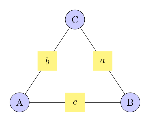
Show Tikz code
print(fig)% --------------------------------------------- %% Tikzfigure generated by tikzfigure v0.3.1 %% https://github.com/max-models/tikzfigure %% --------------------------------------------- %\begin{tikzpicture}[every node/.append style={draw, minimum size=0.7cm}] \node[shape=circle, fill=blue!20] (A) at ({0}, {0}) {A}; \node[shape=circle, fill=blue!20] (B) at ({4}, {0}) {B}; \node[shape=circle, fill=blue!20] (C) at ({2}, {3}) {C}; \draw[color=black] (A) to (B); \draw[color=black] (B) to (C); \draw[color=black] (A) to (C); \node[fill=yellow!60, draw=none] (AB) at ({2.0}, {0.0}) {$c$}; \node[fill=yellow!60, draw=none] (BC) at ({3.0}, {1.5}) {$a$}; \node[fill=yellow!60, draw=none] (AC) at ({1.0}, {1.5}) {$b$};\end{tikzpicture}print(fig.generate_standalone())\documentclass[border=10pt]{standalone}\PassOptionsToPackage{dvipsnames,svgnames,x11names}{xcolor}\usepackage{tikz}\usepackage{pgfplots}\pgfplotsset{compat=newest}\usepgfplotslibrary{groupplots}\usetikzlibrary{arrows.meta}\begin{document}% --------------------------------------------- %% Tikzfigure generated by tikzfigure v0.3.1 %% https://github.com/max-models/tikzfigure %% --------------------------------------------- %\begin{tikzpicture}[every node/.append style={draw, minimum size=0.7cm}] \node[shape=circle, fill=blue!20] (A) at ({0}, {0}) {A}; \node[shape=circle, fill=blue!20] (B) at ({4}, {0}) {B}; \node[shape=circle, fill=blue!20] (C) at ({2}, {3}) {C}; \draw[color=black] (A) to (B); \draw[color=black] (B) to (C); \draw[color=black] (A) to (C); \node[fill=yellow!60, draw=none] (AB) at ({2.0}, {0.0}) {$c$}; \node[fill=yellow!60, draw=none] (BC) at ({3.0}, {1.5}) {$a$}; \node[fill=yellow!60, draw=none] (AC) at ({1.0}, {1.5}) {$b$};\end{tikzpicture}
\end{document}Recursive bisection
Section titled “Recursive bisection”Repeatedly calling midpoint bisects a segment. Here we produce three
levels of binary subdivision.
fig = TikzFigure()
dot = dict(    shape="circle",    minimum_size="6pt",    fill="black",    draw="black",    inner_sep="0pt",    content="",)
left = fig.node(    (0, 0),    label="L",    **dot,)right = fig.node(    (8, 0),    label="R",    **dot,)fig.draw([left, right], color="gray")
m1 = fig.midpoint(    left,    right,    label="M1",    **dot,)m2a = fig.midpoint(    left,    m1,    label="M2a",    **dot,)m2b = fig.midpoint(    m1,    right,    label="M2b",    **dot,)
fig.midpoint(    left,    m2a,    label="M3a",    **dot,)fig.midpoint(    m2a,    m1,    label="M3b",    **dot,)fig.midpoint(    m1,    m2b,    label="M3c",    **dot,)fig.midpoint(    m2b,    right,    label="M3d",    **dot,)
fig.show()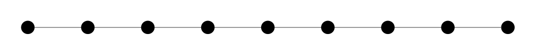
Show Tikz code
print(fig)% --------------------------------------------- %% Tikzfigure generated by tikzfigure v0.3.1 %% https://github.com/max-models/tikzfigure %% --------------------------------------------- %\begin{tikzpicture} \node[shape=circle, fill=black, draw=black, minimum size=6pt, inner sep=0pt] (L) at ({0}, {0}) {}; \node[shape=circle, fill=black, draw=black, minimum size=6pt, inner sep=0pt] (R) at ({8}, {0}) {}; \draw[color=gray] (L) to (R); \node[shape=circle, fill=black, draw=black, minimum size=6pt, inner sep=0pt] (M1) at ({4.0}, {0.0}) {}; \node[shape=circle, fill=black, draw=black, minimum size=6pt, inner sep=0pt] (M2a) at ({2.0}, {0.0}) {}; \node[shape=circle, fill=black, draw=black, minimum size=6pt, inner sep=0pt] (M2b) at ({6.0}, {0.0}) {}; \node[shape=circle, fill=black, draw=black, minimum size=6pt, inner sep=0pt] (M3a) at ({1.0}, {0.0}) {}; \node[shape=circle, fill=black, draw=black, minimum size=6pt, inner sep=0pt] (M3b) at ({3.0}, {0.0}) {}; \node[shape=circle, fill=black, draw=black, minimum size=6pt, inner sep=0pt] (M3c) at ({5.0}, {0.0}) {}; \node[shape=circle, fill=black, draw=black, minimum size=6pt, inner sep=0pt] (M3d) at ({7.0}, {0.0}) {};\end{tikzpicture}print(fig.generate_standalone())\documentclass[border=10pt]{standalone}\PassOptionsToPackage{dvipsnames,svgnames,x11names}{xcolor}\usepackage{tikz}\usepackage{pgfplots}\pgfplotsset{compat=newest}\usepgfplotslibrary{groupplots}\usetikzlibrary{arrows.meta}\begin{document}% --------------------------------------------- %% Tikzfigure generated by tikzfigure v0.3.1 %% https://github.com/max-models/tikzfigure %% --------------------------------------------- %\begin{tikzpicture} \node[shape=circle, fill=black, draw=black, minimum size=6pt, inner sep=0pt] (L) at ({0}, {0}) {}; \node[shape=circle, fill=black, draw=black, minimum size=6pt, inner sep=0pt] (R) at ({8}, {0}) {}; \draw[color=gray] (L) to (R); \node[shape=circle, fill=black, draw=black, minimum size=6pt, inner sep=0pt] (M1) at ({4.0}, {0.0}) {}; \node[shape=circle, fill=black, draw=black, minimum size=6pt, inner sep=0pt] (M2a) at ({2.0}, {0.0}) {}; \node[shape=circle, fill=black, draw=black, minimum size=6pt, inner sep=0pt] (M2b) at ({6.0}, {0.0}) {}; \node[shape=circle, fill=black, draw=black, minimum size=6pt, inner sep=0pt] (M3a) at ({1.0}, {0.0}) {}; \node[shape=circle, fill=black, draw=black, minimum size=6pt, inner sep=0pt] (M3b) at ({3.0}, {0.0}) {}; \node[shape=circle, fill=black, draw=black, minimum size=6pt, inner sep=0pt] (M3c) at ({5.0}, {0.0}) {}; \node[shape=circle, fill=black, draw=black, minimum size=6pt, inner sep=0pt] (M3d) at ({7.0}, {0.0}) {};\end{tikzpicture}
\end{document}Triangle centroid via iterated midpoints
Section titled “Triangle centroid via iterated midpoints”The centroid of a triangle satisfies . We can reach it with two midpoint calls:
(This is equivalent to taking 2/3 along the median from to the midpoint of .)
fig = TikzFigure()
A = fig.node(    (0, 0),    label="A",    content="$A$",    shape="circle",    fill="blue!20",    draw="blue",)B = fig.node(    (6, 0),    label="B",    content="$B$",    shape="circle",    fill="blue!20",    draw="blue",)C = fig.node(    (2, 4),    label="C",    content="$C$",    shape="circle",    fill="blue!20",    draw="blue",)
fig.draw(    [A.center, "B", "C"],    center=True,    cycle=True,    color="blue",    fill="blue!10",    line_width="1.5pt",)
# Midpoint of BC - used to draw the median from Amid_BC = fig.midpoint(    B,    C,    label="MBC",    content="",    shape="circle",    minimum_size="4pt",    fill="gray",    draw="gray",    inner_sep="0pt",)fig.draw([A, mid_BC], options=[styles.dashed], color="gray")
# Centroid = midpoint(midpoint(A, B), C)centroid = fig.midpoint(    fig.midpoint(        A,        B,        label="_MAB",        content="",    ),    C,    label="G",    content="$G$",    shape="circle",    fill="red!60",    draw="red",)
fig.show()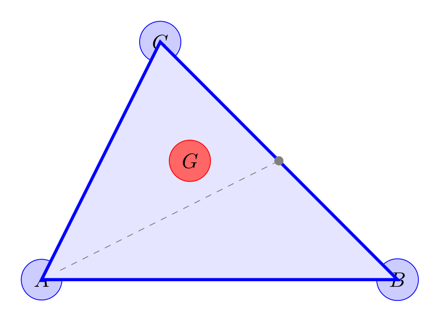
Show Tikz code
print(fig)% --------------------------------------------- %% Tikzfigure generated by tikzfigure v0.3.1 %% https://github.com/max-models/tikzfigure %% --------------------------------------------- %\begin{tikzpicture} \node[shape=circle, fill=blue!20, draw=blue] (A) at ({0}, {0}) {$A$}; \node[shape=circle, fill=blue!20, draw=blue] (B) at ({6}, {0}) {$B$}; \node[shape=circle, fill=blue!20, draw=blue] (C) at ({2}, {4}) {$C$}; \draw[color=blue, fill=blue!10, line width=1.5pt] (A.center) to (B.center) to (C.center) -- cycle; \node[shape=circle, fill=gray, draw=gray, minimum size=4pt, inner sep=0pt] (MBC) at ({4.0}, {2.0}) {}; \draw[dashed, color=gray] (A) to (MBC); \node (_MAB) at ({3.0}, {0.0}) {}; \node[shape=circle, fill=red!60, draw=red] (G) at ({2.5}, {2.0}) {$G$};\end{tikzpicture}print(fig.generate_standalone())\documentclass[border=10pt]{standalone}\PassOptionsToPackage{dvipsnames,svgnames,x11names}{xcolor}\usepackage{tikz}\usepackage{pgfplots}\pgfplotsset{compat=newest}\usepgfplotslibrary{groupplots}\usetikzlibrary{arrows.meta}\begin{document}% --------------------------------------------- %% Tikzfigure generated by tikzfigure v0.3.1 %% https://github.com/max-models/tikzfigure %% --------------------------------------------- %\begin{tikzpicture} \node[shape=circle, fill=blue!20, draw=blue] (A) at ({0}, {0}) {$A$}; \node[shape=circle, fill=blue!20, draw=blue] (B) at ({6}, {0}) {$B$}; \node[shape=circle, fill=blue!20, draw=blue] (C) at ({2}, {4}) {$C$}; \draw[color=blue, fill=blue!10, line width=1.5pt] (A.center) to (B.center) to (C.center) -- cycle; \node[shape=circle, fill=gray, draw=gray, minimum size=4pt, inner sep=0pt] (MBC) at ({4.0}, {2.0}) {}; \draw[dashed, color=gray] (A) to (MBC); \node (_MAB) at ({3.0}, {0.0}) {}; \node[shape=circle, fill=red!60, draw=red] (G) at ({2.5}, {2.0}) {$G$};\end{tikzpicture}
\end{document}Named coordinates as path waypoints
Section titled “Named coordinates as path waypoints”fig.coordinate(label, x, y) plants an invisible named point — no box,
no content, no border. It emits \coordinate (label) at (x,y); in TikZ
and can be referenced in any path list just like a node label.
This is lighter than fig.node() when you only need a reusable
geometric anchor, not a visible element.
fig = TikzFigure()
# Four invisible corners of a diamondfig.coordinate("top", x=3, y=4)fig.coordinate("right", x=6, y=2)fig.coordinate("bot", x=3, y=0)fig.coordinate("left", x=0, y=2)
# Draw a diamond outline and its diagonalsfig.draw(    ["top", "right", "bot", "left"],    cycle=True,    color="teal",    line_width=2,)fig.draw(    ["top", "bot"],    options=[styles.dashed],    color="gray",)fig.draw(    ["left", "right"],    options=[styles.dashed],    color="gray",)
# A visible centre node for referencefig.node(    (3, 2),    content="centre",    draw="none",    font=r"\small",)
fig.show()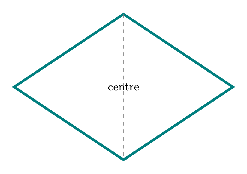
Show Tikz code
print(fig)% --------------------------------------------- %% Tikzfigure generated by tikzfigure v0.3.1 %% https://github.com/max-models/tikzfigure %% --------------------------------------------- %\begin{tikzpicture} \coordinate (top) at ({3}, {4}); \coordinate (right) at ({6}, {2}); \coordinate (bot) at ({3}, {0}); \coordinate (left) at ({0}, {2}); \draw[color=teal, line width=2] (top) to (right) to (bot) to (left) -- cycle; \draw[dashed, color=gray] (top) to (bot); \draw[dashed, color=gray] (left) to (right); \node[draw=none, font=\small] (node0) at ({3}, {2}) {centre};\end{tikzpicture}print(fig.generate_standalone())\documentclass[border=10pt]{standalone}\PassOptionsToPackage{dvipsnames,svgnames,x11names}{xcolor}\usepackage{tikz}\usepackage{pgfplots}\pgfplotsset{compat=newest}\usepgfplotslibrary{groupplots}\usetikzlibrary{arrows.meta}\begin{document}% --------------------------------------------- %% Tikzfigure generated by tikzfigure v0.3.1 %% https://github.com/max-models/tikzfigure %% --------------------------------------------- %\begin{tikzpicture} \coordinate (top) at ({3}, {4}); \coordinate (right) at ({6}, {2}); \coordinate (bot) at ({3}, {0}); \coordinate (left) at ({0}, {2}); \draw[color=teal, line width=2] (top) to (right) to (bot) to (left) -- cycle; \draw[dashed, color=gray] (top) to (bot); \draw[dashed, color=gray] (left) to (right); \node[draw=none, font=\small] (node0) at ({3}, {2}) {centre};\end{tikzpicture}
\end{document}Routing paths via intermediate coordinates
Section titled “Routing paths via intermediate coordinates”A common TikZ pattern is bending a connection around an obstacle by routing it through an invisible corner coordinate. Here two nodes are connected with an L-shaped arrow: the path goes horizontally to a corner, then vertically up.
fig = TikzFigure()
fig.node(    (0, 0),    label="src",    shape="rectangle",    draw="blue!70",    fill="blue!15",    minimum_width="1.8cm",    minimum_height="0.8cm",    content="source",)fig.node(    (5, 3),    label="dst",    shape="rectangle",    draw="orange!80",    fill="orange!15",    minimum_width="1.8cm",    minimum_height="0.8cm",    content="dest",)
# Corner at the same column as dst, same row as srcfig.coordinate("corner", x=5, y=0)
fig.draw(    ["src.east", "corner", "dst.south"],    arrows=arrows.forward,    options=[styles.thick],    color="purple",    segment_options=[        {"connector": "--"},  # horizontal segment: straight line        {"connector": "--"},  # vertical segment: straight line    ],)
fig.show()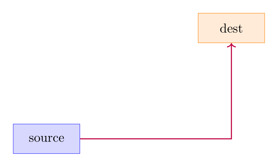
Show Tikz code
print(fig)% --------------------------------------------- %% Tikzfigure generated by tikzfigure v0.3.1 %% https://github.com/max-models/tikzfigure %% --------------------------------------------- %\begin{tikzpicture} \node[shape=rectangle, fill=blue!15, draw=blue!70, minimum width=1.8cm, minimum height=0.8cm] (src) at ({0}, {0}) {source}; \node[shape=rectangle, fill=orange!15, draw=orange!80, minimum width=1.8cm, minimum height=0.8cm] (dst) at ({5}, {3}) {dest}; \coordinate (corner) at ({5}, {0}); \draw[thick, ->, color=purple] (src.east) -- (corner) -- (dst.south);\end{tikzpicture}print(fig.generate_standalone())\documentclass[border=10pt]{standalone}\PassOptionsToPackage{dvipsnames,svgnames,x11names}{xcolor}\usepackage{tikz}\usepackage{pgfplots}\pgfplotsset{compat=newest}\usepgfplotslibrary{groupplots}\usetikzlibrary{arrows.meta}\begin{document}% --------------------------------------------- %% Tikzfigure generated by tikzfigure v0.3.1 %% https://github.com/max-models/tikzfigure %% --------------------------------------------- %\begin{tikzpicture} \node[shape=rectangle, fill=blue!15, draw=blue!70, minimum width=1.8cm, minimum height=0.8cm] (src) at ({0}, {0}) {source}; \node[shape=rectangle, fill=orange!15, draw=orange!80, minimum width=1.8cm, minimum height=0.8cm] (dst) at ({5}, {3}) {dest}; \coordinate (corner) at ({5}, {0}); \draw[thick, ->, color=purple] (src.east) -- (corner) -- (dst.south);\end{tikzpicture}
\end{document}Coordinates from expressions (calc library)
Section titled “Coordinates from expressions (calc library)”When you add \usetikzlibrary{calc} via document_setup, the at
parameter of fig.coordinate() accepts full calc expressions. The
$(A)!t!(B)$ syntax places a point a fraction t of the way from A
to B.
fig = TikzFigure()fig.usetikzlibrary("calc")
fig.node(    (0, 0),    label="A",    shape="circle",    fill="blue!20",    draw="blue!70",    minimum_size="1cm",    content="$A$",)fig.node(    (8, 0),    label="B",    shape="circle",    fill="red!20",    draw="red!70",    minimum_size="1cm",    content="$B$",)fig.node(    (4, 5),    label="C",    shape="circle",    fill="green!20",    draw="green!70",    minimum_size="1cm",    content="$C$",)
# Invisible midpoints of each edge using calc expressionsfig.coordinate("mAB", at="$(A)!0.5!(B)$")fig.coordinate("mBC", at="$(B)!0.5!(C)$")fig.coordinate("mCA", at="$(C)!0.5!(A)$")
# Outline trianglefig.draw(    ["A.center", "B.center", "C.center"],    cycle=True,    color="gray!50",    line_width=1,)
# Medial triangle connecting the three edge midpointsfig.draw(    ["mAB", "mBC", "mCA"],    cycle=True,    color="purple",    line_width=2,    fill="purple!10",    fill_opacity=0.5,)
fig.show()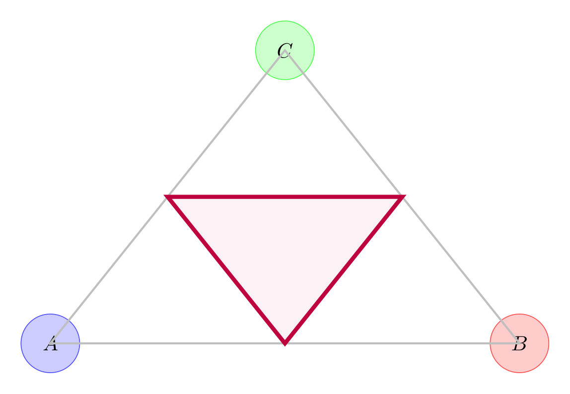
Show Tikz code
print(fig)% --------------------------------------------- %% Tikzfigure generated by tikzfigure v0.3.1 %% https://github.com/max-models/tikzfigure %% --------------------------------------------- %\begin{tikzpicture} \node[shape=circle, fill=blue!20, draw=blue!70, minimum size=1cm] (A) at ({0}, {0}) {$A$}; \node[shape=circle, fill=red!20, draw=red!70, minimum size=1cm] (B) at ({8}, {0}) {$B$}; \node[shape=circle, fill=green!20, draw=green!70, minimum size=1cm] (C) at ({4}, {5}) {$C$}; \coordinate (mAB) at ($(A)!0.5!(B)$); \coordinate (mBC) at ($(B)!0.5!(C)$); \coordinate (mCA) at ($(C)!0.5!(A)$); \draw[color=gray!50, line width=1] (A.center) to (B.center) to (C.center) -- cycle; \draw[color=purple, fill=purple!10, fill opacity=0.5, line width=2] (mAB) to (mBC) to (mCA) -- cycle;\end{tikzpicture}print(fig.generate_standalone())\documentclass[border=10pt]{standalone}\PassOptionsToPackage{dvipsnames,svgnames,x11names}{xcolor}\usepackage{tikz}\usepackage{pgfplots}\pgfplotsset{compat=newest}\usepgfplotslibrary{groupplots}\usetikzlibrary{arrows.meta,calc}\begin{document}% --------------------------------------------- %% Tikzfigure generated by tikzfigure v0.3.1 %% https://github.com/max-models/tikzfigure %% --------------------------------------------- %\begin{tikzpicture} \node[shape=circle, fill=blue!20, draw=blue!70, minimum size=1cm] (A) at ({0}, {0}) {$A$}; \node[shape=circle, fill=red!20, draw=red!70, minimum size=1cm] (B) at ({8}, {0}) {$B$}; \node[shape=circle, fill=green!20, draw=green!70, minimum size=1cm] (C) at ({4}, {5}) {$C$}; \coordinate (mAB) at ($(A)!0.5!(B)$); \coordinate (mBC) at ($(B)!0.5!(C)$); \coordinate (mCA) at ($(C)!0.5!(A)$); \draw[color=gray!50, line width=1] (A.center) to (B.center) to (C.center) -- cycle; \draw[color=purple, fill=purple!10, fill opacity=0.5, line width=2] (mAB) to (mBC) to (mCA) -- cycle;\end{tikzpicture}
\end{document}