2D Plots: Functions
pgfplots can evaluate mathematical functions directly, and Python’s
math module gives you full flexibility for data generation.
import mathfrom tikzfigure import TikzFigurePlotting functions directly
Section titled “Plotting functions directly”Pass a function expression as a string to func= for smooth curves
without pre-computing data points:
fig = TikzFigure()
ax = fig.axis2d(    xlabel="x",    ylabel="y",    xlim=(0, 360),    ylim=(-1.5, 1.5),    grid=True,)
ax.add_plot(    func="sin(x)",    label=r"$\sin(x)$",    color="red",    line_width="1.5pt",)ax.add_plot(    func="cos(x)",    label=r"$\cos(x)$",    color="blue",    line_width="1.5pt",)
ax.set_legend(position="south east")fig.show()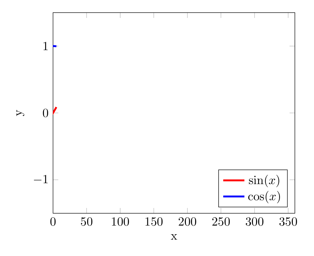
Show Tikz code
print(fig)% --------------------------------------------- %% Tikzfigure generated by tikzfigure v0.3.1 %% https://github.com/max-models/tikzfigure %% --------------------------------------------- %\begin{tikzpicture} \begin{axis}[xlabel=x, ylabel=y, xmin=0, xmax=360, ymin=-1.5, ymax=1.5, grid=major, legend pos=south east] \addplot[color=red, line width=1.5pt] {sin(x)}; \addplot[color=blue, line width=1.5pt] {cos(x)}; \legend{$\sin(x)$, $\cos(x)$} \end{axis}\end{tikzpicture}print(fig.generate_standalone())\documentclass[border=10pt]{standalone}\PassOptionsToPackage{dvipsnames,svgnames,x11names}{xcolor}\usepackage{tikz}\usepackage{pgfplots}\pgfplotsset{compat=newest}\usepgfplotslibrary{groupplots}\usetikzlibrary{arrows.meta}\usepackage{pgfplots}\begin{document}% --------------------------------------------- %% Tikzfigure generated by tikzfigure v0.3.1 %% https://github.com/max-models/tikzfigure %% --------------------------------------------- %\begin{tikzpicture} \begin{axis}[xlabel=x, ylabel=y, xmin=0, xmax=360, ymin=-1.5, ymax=1.5, grid=major, legend pos=south east] \addplot[color=red, line width=1.5pt] {sin(x)}; \addplot[color=blue, line width=1.5pt] {cos(x)}; \legend{$\sin(x)$, $\cos(x)$} \end{axis}\end{tikzpicture}
\end{document}func accepts any pgfplots expression: sin(x), cos(x), x^2,
sqrt(x), exp(x), ln(x), etc.
Comparing functions
Section titled “Comparing functions”Plot multiple functions side-by-side:
fig = TikzFigure()
ax = fig.axis2d(    xlabel="$x$",    ylabel="$y$",    xlim=(0, 10),    ylim=(0, 5),    grid=True,)
ax.add_plot(func="x", label="$x$", color="black")ax.add_plot(    func="sqrt(x)",    label=r"$\sqrt{x}$",    color="blue",    line_width="2pt",)ax.add_plot(    func="x/2",    label="$x/2$",    color="green",)
ax.set_legend(position="north west")fig.show()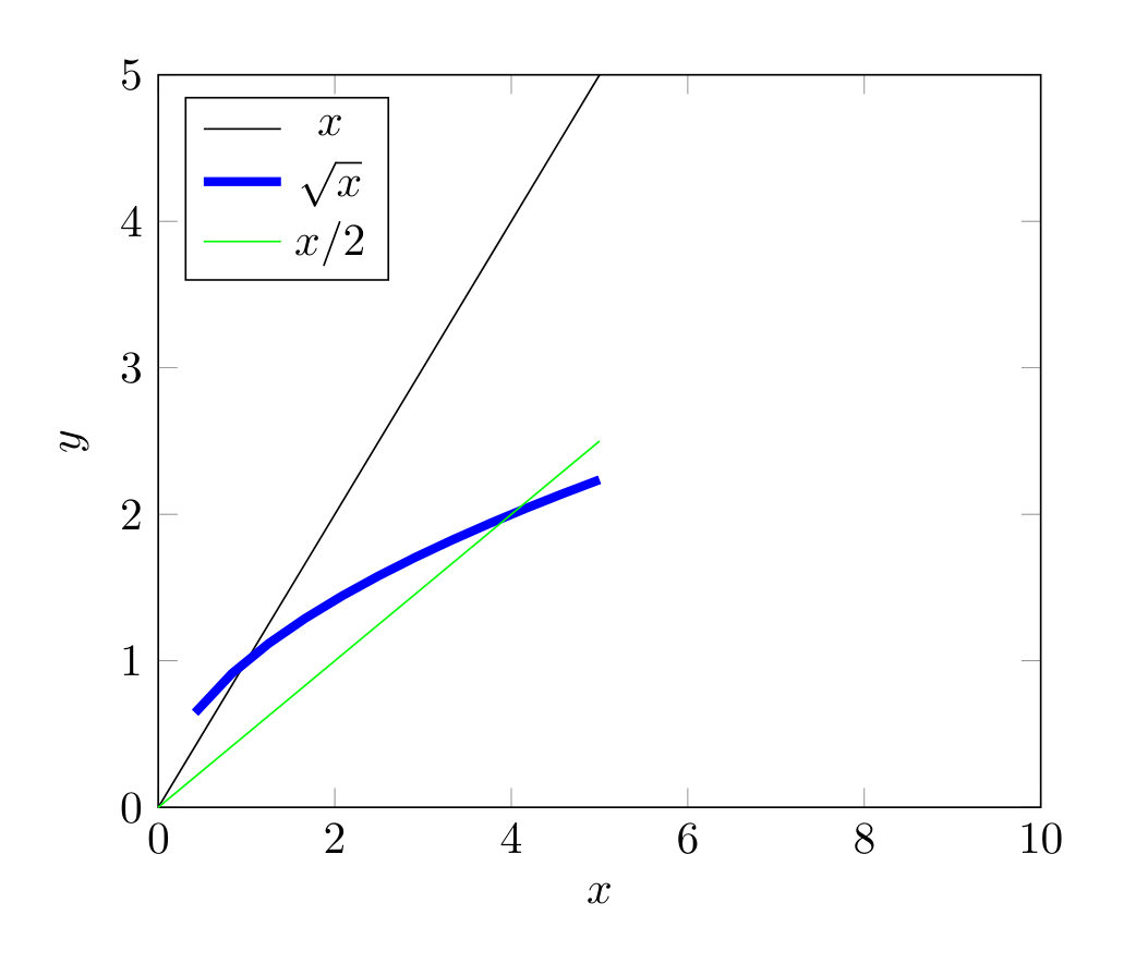
Show Tikz code
print(fig)% --------------------------------------------- %% Tikzfigure generated by tikzfigure v0.3.1 %% https://github.com/max-models/tikzfigure %% --------------------------------------------- %\begin{tikzpicture} \begin{axis}[xlabel=$x$, ylabel=$y$, xmin=0, xmax=10, ymin=0, ymax=5, grid=major, legend pos=north west] \addplot[color=black] {x}; \addplot[color=blue, line width=2pt] {sqrt(x)}; \addplot[color=green] {x/2}; \legend{$x$, $\sqrt{x}$, $x/2$} \end{axis}\end{tikzpicture}print(fig.generate_standalone())\documentclass[border=10pt]{standalone}\PassOptionsToPackage{dvipsnames,svgnames,x11names}{xcolor}\usepackage{tikz}\usepackage{pgfplots}\pgfplotsset{compat=newest}\usepgfplotslibrary{groupplots}\usetikzlibrary{arrows.meta}\usepackage{pgfplots}\begin{document}% --------------------------------------------- %% Tikzfigure generated by tikzfigure v0.3.1 %% https://github.com/max-models/tikzfigure %% --------------------------------------------- %\begin{tikzpicture} \begin{axis}[xlabel=$x$, ylabel=$y$, xmin=0, xmax=10, ymin=0, ymax=5, grid=major, legend pos=north west] \addplot[color=black] {x}; \addplot[color=blue, line width=2pt] {sqrt(x)}; \addplot[color=green] {x/2}; \legend{$x$, $\sqrt{x}$, $x/2$} \end{axis}\end{tikzpicture}
\end{document}Generating data with Python
Section titled “Generating data with Python”For more complex curves, use Python’s math module with list
comprehensions:
fig = TikzFigure()
ax = fig.axis2d(    xlabel="Angle (radians)",    ylabel="Amplitude",    xlim=(0, 6.5),    ylim=(-1.5, 1.5),    grid=True,)
x = [i * 0.1 for i in range(65)]y_sin = [math.sin(xi) for xi in x]y_cos = [math.cos(xi) for xi in x]
ax.add_plot(    x,    y_sin,    label=r"$\sin(x)$",    color="red",)ax.add_plot(    x,    y_cos,    label=r"$\cos(x)$",    color="blue",)
ax.set_legend(position="south east")fig.show()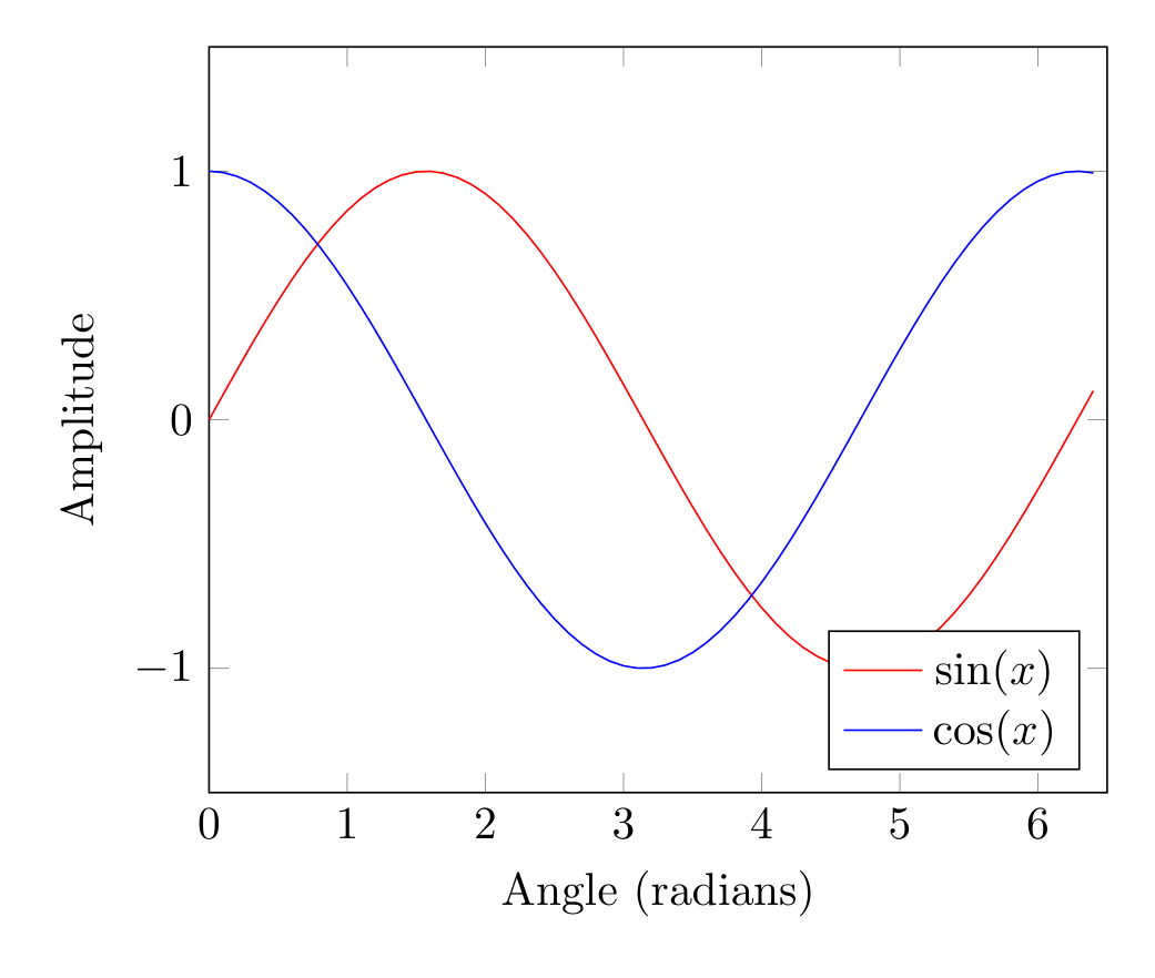
Show Tikz code
print(fig)% --------------------------------------------- %% Tikzfigure generated by tikzfigure v0.3.1 %% https://github.com/max-models/tikzfigure %% --------------------------------------------- %\begin{tikzpicture} \begin{axis}[xlabel=Angle (radians), ylabel=Amplitude, xmin=0, xmax=6.5, ymin=-1.5, ymax=1.5, grid=major, legend pos=south east] \addplot[color=red] coordinates {(0.0,0.0) (0.1,0.09983341664682815) (0.2,0.19866933079506122) (0.30000000000000004,0.2955202066613396) (0.4,0.3894183423086505) (0.5,0.479425538604203) (0.6000000000000001,0.5646424733950355) (0.7000000000000001,0.6442176872376911) (0.8,0.7173560908995228) (0.9,0.7833269096274834) (1.0,0.8414709848078965) (1.1,0.8912073600614354) (1.2000000000000002,0.9320390859672264) (1.3,0.963558185417193) (1.4000000000000001,0.9854497299884603) (1.5,0.9974949866040544) (1.6,0.9995736030415051) (1.7000000000000002,0.9916648104524686) (1.8,0.9738476308781951) (1.9000000000000001,0.9463000876874145) (2.0,0.9092974268256817) (2.1,0.8632093666488737) (2.2,0.8084964038195901) (2.3000000000000003,0.74570521217672) (2.4000000000000004,0.6754631805511506) (2.5,0.5984721441039565) (2.6,0.5155013718214642) (2.7,0.4273798802338298) (2.8000000000000003,0.33498815015590466) (2.9000000000000004,0.23924932921398198) (3.0,0.1411200080598672) (3.1,0.04158066243329049) (3.2,-0.058374143427580086) (3.3000000000000003,-0.15774569414324865) (3.4000000000000004,-0.25554110202683167) (3.5,-0.35078322768961984) (3.6,-0.44252044329485246) (3.7,-0.5298361409084934) (3.8000000000000003,-0.6118578909427193) (3.9000000000000004,-0.6877661591839741) (4.0,-0.7568024953079282) (4.1000000000000005,-0.8182771110644108) (4.2,-0.8715757724135882) (4.3,-0.9161659367494549) (4.4,-0.951602073889516) (4.5,-0.977530117665097) (4.6000000000000005,-0.9936910036334645) (4.7,-0.9999232575641008) (4.800000000000001,-0.9961646088358406) (4.9,-0.9824526126243325) (5.0,-0.9589242746631385) (5.1000000000000005,-0.9258146823277321) (5.2,-0.8834546557201531) (5.300000000000001,-0.8322674422239008) (5.4,-0.7727644875559871) (5.5,-0.7055403255703919) (5.6000000000000005,-0.6312666378723208) (5.7,-0.5506855425976376) (5.800000000000001,-0.4646021794137566) (5.9,-0.373876664830236) (6.0,-0.27941549819892586) (6.1000000000000005,-0.18216250427209502) (6.2,-0.0830894028174964) (6.300000000000001,0.0168139004843506) (6.4,0.11654920485049364)}; \addplot[color=blue] coordinates {(0.0,1.0) (0.1,0.9950041652780258) (0.2,0.9800665778412416) (0.30000000000000004,0.955336489125606) (0.4,0.9210609940028851) (0.5,0.8775825618903728) (0.6000000000000001,0.8253356149096782) (0.7000000000000001,0.7648421872844884) (0.8,0.6967067093471654) (0.9,0.6216099682706644) (1.0,0.5403023058681398) (1.1,0.4535961214255773) (1.2000000000000002,0.3623577544766734) (1.3,0.26749882862458735) (1.4000000000000001,0.16996714290024081) (1.5,0.0707372016677029) (1.6,-0.029199522301288815) (1.7000000000000002,-0.12884449429552486) (1.8,-0.2272020946930871) (1.9000000000000001,-0.3232895668635036) (2.0,-0.4161468365471424) (2.1,-0.5048461045998576) (2.2,-0.5885011172553458) (2.3000000000000003,-0.6662760212798244) (2.4000000000000004,-0.7373937155412458) (2.5,-0.8011436155469337) (2.6,-0.8568887533689473) (2.7,-0.9040721420170612) (2.8000000000000003,-0.9422223406686583) (2.9000000000000004,-0.9709581651495907) (3.0,-0.9899924966004454) (3.1,-0.9991351502732795) (3.2,-0.9982947757947531) (3.3000000000000003,-0.9874797699088649) (3.4000000000000004,-0.9667981925794609) (3.5,-0.9364566872907963) (3.6,-0.896758416334147) (3.7,-0.848100031710408) (3.8000000000000003,-0.7909677119144165) (3.9000000000000004,-0.7259323042001399) (4.0,-0.6536436208636119) (4.1000000000000005,-0.5748239465332685) (4.2,-0.4902608213406994) (4.3,-0.40079917207997545) (4.4,-0.30733286997841935) (4.5,-0.2107957994307797) (4.6000000000000005,-0.11215252693505398) (4.7,-0.01238866346289056) (4.800000000000001,0.08749898343944727) (4.9,0.18651236942257576) (5.0,0.28366218546322625) (5.1000000000000005,0.37797774271298107) (5.2,0.4685166713003771) (5.300000000000001,0.5543743361791615) (5.4,0.6346928759426347) (5.5,0.70866977429126) (5.6000000000000005,0.7755658785102502) (5.7,0.8347127848391598) (5.800000000000001,0.8855195169413194) (5.9,0.9274784307440359) (6.0,0.960170286650366) (6.1000000000000005,0.9832684384425847) (6.2,0.9965420970232175) (6.300000000000001,0.9998586363834151) (6.4,0.9931849187581926)}; \legend{$\sin(x)$, $\cos(x)$} \end{axis}\end{tikzpicture}print(fig.generate_standalone())\documentclass[border=10pt]{standalone}\PassOptionsToPackage{dvipsnames,svgnames,x11names}{xcolor}\usepackage{tikz}\usepackage{pgfplots}\pgfplotsset{compat=newest}\usepgfplotslibrary{groupplots}\usetikzlibrary{arrows.meta}\usepackage{pgfplots}\begin{document}% --------------------------------------------- %% Tikzfigure generated by tikzfigure v0.3.1 %% https://github.com/max-models/tikzfigure %% --------------------------------------------- %\begin{tikzpicture} \begin{axis}[xlabel=Angle (radians), ylabel=Amplitude, xmin=0, xmax=6.5, ymin=-1.5, ymax=1.5, grid=major, legend pos=south east] \addplot[color=red] coordinates {(0.0,0.0) (0.1,0.09983341664682815) (0.2,0.19866933079506122) (0.30000000000000004,0.2955202066613396) (0.4,0.3894183423086505) (0.5,0.479425538604203) (0.6000000000000001,0.5646424733950355) (0.7000000000000001,0.6442176872376911) (0.8,0.7173560908995228) (0.9,0.7833269096274834) (1.0,0.8414709848078965) (1.1,0.8912073600614354) (1.2000000000000002,0.9320390859672264) (1.3,0.963558185417193) (1.4000000000000001,0.9854497299884603) (1.5,0.9974949866040544) (1.6,0.9995736030415051) (1.7000000000000002,0.9916648104524686) (1.8,0.9738476308781951) (1.9000000000000001,0.9463000876874145) (2.0,0.9092974268256817) (2.1,0.8632093666488737) (2.2,0.8084964038195901) (2.3000000000000003,0.74570521217672) (2.4000000000000004,0.6754631805511506) (2.5,0.5984721441039565) (2.6,0.5155013718214642) (2.7,0.4273798802338298) (2.8000000000000003,0.33498815015590466) (2.9000000000000004,0.23924932921398198) (3.0,0.1411200080598672) (3.1,0.04158066243329049) (3.2,-0.058374143427580086) (3.3000000000000003,-0.15774569414324865) (3.4000000000000004,-0.25554110202683167) (3.5,-0.35078322768961984) (3.6,-0.44252044329485246) (3.7,-0.5298361409084934) (3.8000000000000003,-0.6118578909427193) (3.9000000000000004,-0.6877661591839741) (4.0,-0.7568024953079282) (4.1000000000000005,-0.8182771110644108) (4.2,-0.8715757724135882) (4.3,-0.9161659367494549) (4.4,-0.951602073889516) (4.5,-0.977530117665097) (4.6000000000000005,-0.9936910036334645) (4.7,-0.9999232575641008) (4.800000000000001,-0.9961646088358406) (4.9,-0.9824526126243325) (5.0,-0.9589242746631385) (5.1000000000000005,-0.9258146823277321) (5.2,-0.8834546557201531) (5.300000000000001,-0.8322674422239008) (5.4,-0.7727644875559871) (5.5,-0.7055403255703919) (5.6000000000000005,-0.6312666378723208) (5.7,-0.5506855425976376) (5.800000000000001,-0.4646021794137566) (5.9,-0.373876664830236) (6.0,-0.27941549819892586) (6.1000000000000005,-0.18216250427209502) (6.2,-0.0830894028174964) (6.300000000000001,0.0168139004843506) (6.4,0.11654920485049364)}; \addplot[color=blue] coordinates {(0.0,1.0) (0.1,0.9950041652780258) (0.2,0.9800665778412416) (0.30000000000000004,0.955336489125606) (0.4,0.9210609940028851) (0.5,0.8775825618903728) (0.6000000000000001,0.8253356149096782) (0.7000000000000001,0.7648421872844884) (0.8,0.6967067093471654) (0.9,0.6216099682706644) (1.0,0.5403023058681398) (1.1,0.4535961214255773) (1.2000000000000002,0.3623577544766734) (1.3,0.26749882862458735) (1.4000000000000001,0.16996714290024081) (1.5,0.0707372016677029) (1.6,-0.029199522301288815) (1.7000000000000002,-0.12884449429552486) (1.8,-0.2272020946930871) (1.9000000000000001,-0.3232895668635036) (2.0,-0.4161468365471424) (2.1,-0.5048461045998576) (2.2,-0.5885011172553458) (2.3000000000000003,-0.6662760212798244) (2.4000000000000004,-0.7373937155412458) (2.5,-0.8011436155469337) (2.6,-0.8568887533689473) (2.7,-0.9040721420170612) (2.8000000000000003,-0.9422223406686583) (2.9000000000000004,-0.9709581651495907) (3.0,-0.9899924966004454) (3.1,-0.9991351502732795) (3.2,-0.9982947757947531) (3.3000000000000003,-0.9874797699088649) (3.4000000000000004,-0.9667981925794609) (3.5,-0.9364566872907963) (3.6,-0.896758416334147) (3.7,-0.848100031710408) (3.8000000000000003,-0.7909677119144165) (3.9000000000000004,-0.7259323042001399) (4.0,-0.6536436208636119) (4.1000000000000005,-0.5748239465332685) (4.2,-0.4902608213406994) (4.3,-0.40079917207997545) (4.4,-0.30733286997841935) (4.5,-0.2107957994307797) (4.6000000000000005,-0.11215252693505398) (4.7,-0.01238866346289056) (4.800000000000001,0.08749898343944727) (4.9,0.18651236942257576) (5.0,0.28366218546322625) (5.1000000000000005,0.37797774271298107) (5.2,0.4685166713003771) (5.300000000000001,0.5543743361791615) (5.4,0.6346928759426347) (5.5,0.70866977429126) (5.6000000000000005,0.7755658785102502) (5.7,0.8347127848391598) (5.800000000000001,0.8855195169413194) (5.9,0.9274784307440359) (6.0,0.960170286650366) (6.1000000000000005,0.9832684384425847) (6.2,0.9965420970232175) (6.300000000000001,0.9998586363834151) (6.4,0.9931849187581926)}; \legend{$\sin(x)$, $\cos(x)$} \end{axis}\end{tikzpicture}
\end{document}Exponential growth
Section titled “Exponential growth”Visualizing exponential functions with Python-generated data:
fig = TikzFigure()
ax = fig.axis2d(    xlabel="Time (years)",    ylabel="Population",    xlim=(0, 10),    ylim=(0, 1000),    grid=True,)
time = [i for i in range(11)]population = [100 * math.exp(0.1 * t) for t in time]
ax.add_plot(    time,    population,    label="$P(t) = 100 e^{0.1t}$",    color="darkgreen",    mark="o",    mark_size="2pt",)
ax.set_legend(position="north west")fig.show()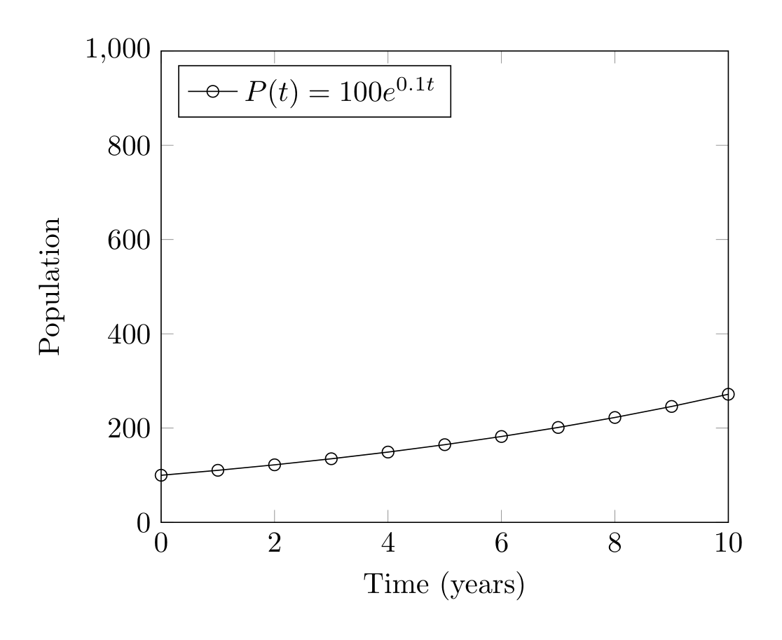
Show Tikz code
print(fig)% --------------------------------------------- %% Tikzfigure generated by tikzfigure v0.3.1 %% https://github.com/max-models/tikzfigure %% --------------------------------------------- %\begin{tikzpicture} \begin{axis}[xlabel=Time (years), ylabel=Population, xmin=0, xmax=10, ymin=0, ymax=1000, grid=major, legend pos=north west] \addplot[color=darkgreen, mark=o, mark size=2pt] coordinates {(0,100.0) (1,110.51709180756477) (2,122.14027581601698) (3,134.9858807576003) (4,149.18246976412703) (5,164.87212707001282) (6,182.21188003905093) (7,201.37527074704767) (8,222.55409284924679) (9,245.960311115695) (10,271.8281828459045)}; \legend{$P(t) = 100 e^{0.1t}$} \end{axis}\end{tikzpicture}print(fig.generate_standalone())\documentclass[border=10pt]{standalone}\PassOptionsToPackage{dvipsnames,svgnames,x11names}{xcolor}\usepackage{tikz}\usepackage{pgfplots}\pgfplotsset{compat=newest}\usepgfplotslibrary{groupplots}\usetikzlibrary{arrows.meta}\usepackage{pgfplots}\begin{document}% --------------------------------------------- %% Tikzfigure generated by tikzfigure v0.3.1 %% https://github.com/max-models/tikzfigure %% --------------------------------------------- %\begin{tikzpicture} \begin{axis}[xlabel=Time (years), ylabel=Population, xmin=0, xmax=10, ymin=0, ymax=1000, grid=major, legend pos=north west] \addplot[color=darkgreen, mark=o, mark size=2pt] coordinates {(0,100.0) (1,110.51709180756477) (2,122.14027581601698) (3,134.9858807576003) (4,149.18246976412703) (5,164.87212707001282) (6,182.21188003905093) (7,201.37527074704767) (8,222.55409284924679) (9,245.960311115695) (10,271.8281828459045)}; \legend{$P(t) = 100 e^{0.1t}$} \end{axis}\end{tikzpicture}
\end{document}