Figure Configuration
TikzFigure accepts several constructor parameters that control how the
figure is set up in LaTeX. This tutorial covers:
figure_setup: global TikZ options applied to the entiretikzpictureenvironmentadd_style(): named TikZ styles at figure scopescope(): local option blocks inside the figuregrid: debug grid overlaydocument_setup: raw LaTeX preamble additions (for\usetikzlibraryetc.)add_package(): additional LaTeX packagesgenerate_standalone(): inspecting the full compilable documentlabel: wrapping the figure in a\begin{figure}environmentfigsize: display-size hint for Jupyter
from tikzfigure import TikzFigure, arrows, stylesfigure_setup: global TikZ options
Section titled “figure_setup: global TikZ options”The figure_setup string is placed inside \begin{tikzpicture}[HERE].
Anything you would normally write in the tikzpicture options block
goes here.
A particularly useful technique is every node/.append style={...} — it
applies a style to every node in the figure without repeating the
options on each individual node call.
fig = TikzFigure(    figure_setup="every node/.append style={draw, fill=blue!10, minimum size=1.2cm}",)
A = fig.node((0, 0), content="A")B = fig.node((2, 0), content="B")C = fig.node((4, 0), content="C")D = fig.node((1, 2), content="D")E = fig.node((3, 2), content="E")
fig.draw([A, B, C], arrows=arrows.forward)fig.draw([D, E], arrows=arrows.forward)
fig.show()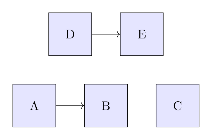
Show Tikz code
print(fig)% --------------------------------------------- %% Tikzfigure generated by tikzfigure v0.3.1 %% https://github.com/max-models/tikzfigure %% --------------------------------------------- %\begin{tikzpicture}[every node/.append style={draw, fill=blue!10, minimum size=1.2cm}] \node (node0) at ({0}, {0}) {A}; \node (node1) at ({2}, {0}) {B}; \node (node2) at ({4}, {0}) {C}; \node (node3) at ({1}, {2}) {D}; \node (node4) at ({3}, {2}) {E}; \draw[->] (node0) to (node1) to (node2); \draw[->] (node3) to (node4);\end{tikzpicture}print(fig.generate_standalone())\documentclass[border=10pt]{standalone}\PassOptionsToPackage{dvipsnames,svgnames,x11names}{xcolor}\usepackage{tikz}\usepackage{pgfplots}\pgfplotsset{compat=newest}\usepgfplotslibrary{groupplots}\usetikzlibrary{arrows.meta}\begin{document}% --------------------------------------------- %% Tikzfigure generated by tikzfigure v0.3.1 %% https://github.com/max-models/tikzfigure %% --------------------------------------------- %\begin{tikzpicture}[every node/.append style={draw, fill=blue!10, minimum size=1.2cm}] \node (node0) at ({0}, {0}) {A}; \node (node1) at ({2}, {0}) {B}; \node (node2) at ({4}, {0}) {C}; \node (node3) at ({1}, {2}) {D}; \node (node4) at ({3}, {2}) {E}; \draw[->] (node0) to (node1) to (node2); \draw[->] (node3) to (node4);\end{tikzpicture}
\end{document}Every node gets a border and blue tint automatically — no per-node
draw= or fill= needed.
# A more elaborate example: uniform rounded rectangles in a flow diagramfig = TikzFigure(    figure_setup=(        "every node/.append style={"        "draw=gray!70, fill=gray!10, "        "minimum width=2cm, minimum height=0.8cm, "        "rounded corners=4pt, font=\\small"        "}"    ),)
nodes = ["Input", "Process", "Output"]for i, label in enumerate(nodes):    fig.node(i * 3, 0, content=label)
for i in range(len(nodes) - 1):    fig.draw(        [(i * 3 + 1.0, 0), (i * 3 + 2.0, 0)],        arrows=arrows.forward,        color="gray!70",    )
fig.show()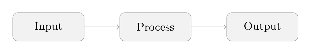
Show Tikz code
print(fig)% --------------------------------------------- %% Tikzfigure generated by tikzfigure v0.3.1 %% https://github.com/max-models/tikzfigure %% --------------------------------------------- %\begin{tikzpicture}[every node/.append style={draw=gray!70, fill=gray!10, minimum width=2cm, minimum height=0.8cm, rounded corners=4pt, font=\small}] \node (node0) at ({0}, {0}) {Input}; \node (node1) at ({3}, {0}) {Process}; \node (node2) at ({6}, {0}) {Output}; \draw[->, color=gray!70] (1.0, 0) to (2.0, 0); \draw[->, color=gray!70] (4.0, 0) to (5.0, 0);\end{tikzpicture}print(fig.generate_standalone())\documentclass[border=10pt]{standalone}\PassOptionsToPackage{dvipsnames,svgnames,x11names}{xcolor}\usepackage{tikz}\usepackage{pgfplots}\pgfplotsset{compat=newest}\usepgfplotslibrary{groupplots}\usetikzlibrary{arrows.meta}\begin{document}% --------------------------------------------- %% Tikzfigure generated by tikzfigure v0.3.1 %% https://github.com/max-models/tikzfigure %% --------------------------------------------- %\begin{tikzpicture}[every node/.append style={draw=gray!70, fill=gray!10, minimum width=2cm, minimum height=0.8cm, rounded corners=4pt, font=\small}] \node (node0) at ({0}, {0}) {Input}; \node (node1) at ({3}, {0}) {Process}; \node (node2) at ({6}, {0}) {Output}; \draw[->, color=gray!70] (1.0, 0) to (2.0, 0); \draw[->, color=gray!70] (4.0, 0) to (5.0, 0);\end{tikzpicture}
\end{document}add_style(): named TikZ styles at figure scope
Section titled “add_style(): named TikZ styles at figure scope”Use add_style() when you want reusable named styles inside the
tikzpicture[...] options block. This is the first-class equivalent of
writing entries such as important line/.style={very thick} by hand.
add_style() returns a reusable style token, so you can immediately
apply the new style in later drawing calls.
fig = TikzFigure()
axes = fig.add_style("axes")important_line = fig.add_style("important line", options=["very thick"])information_text = fig.add_style(    "information text",    options=["rounded corners"],    fill="red!10",    inner_sep="1ex",)
fig.draw(    [(-1, 0), (2, 0)],    options=[axes, arrows.forward],    color="gray!70",)fig.draw(    [(0, -1), (0, 2)],    options=[axes, arrows.forward],    color="gray!70",)fig.draw(    [(0, 0), (1.2, 1.4)],    options=[important_line],    color="blue!70",)fig.node(    (2.3, 1.1),    content="Named styles\nstay reusable",    options=[information_text],    text_width="3.2cm",    anchor="west",)
fig.show()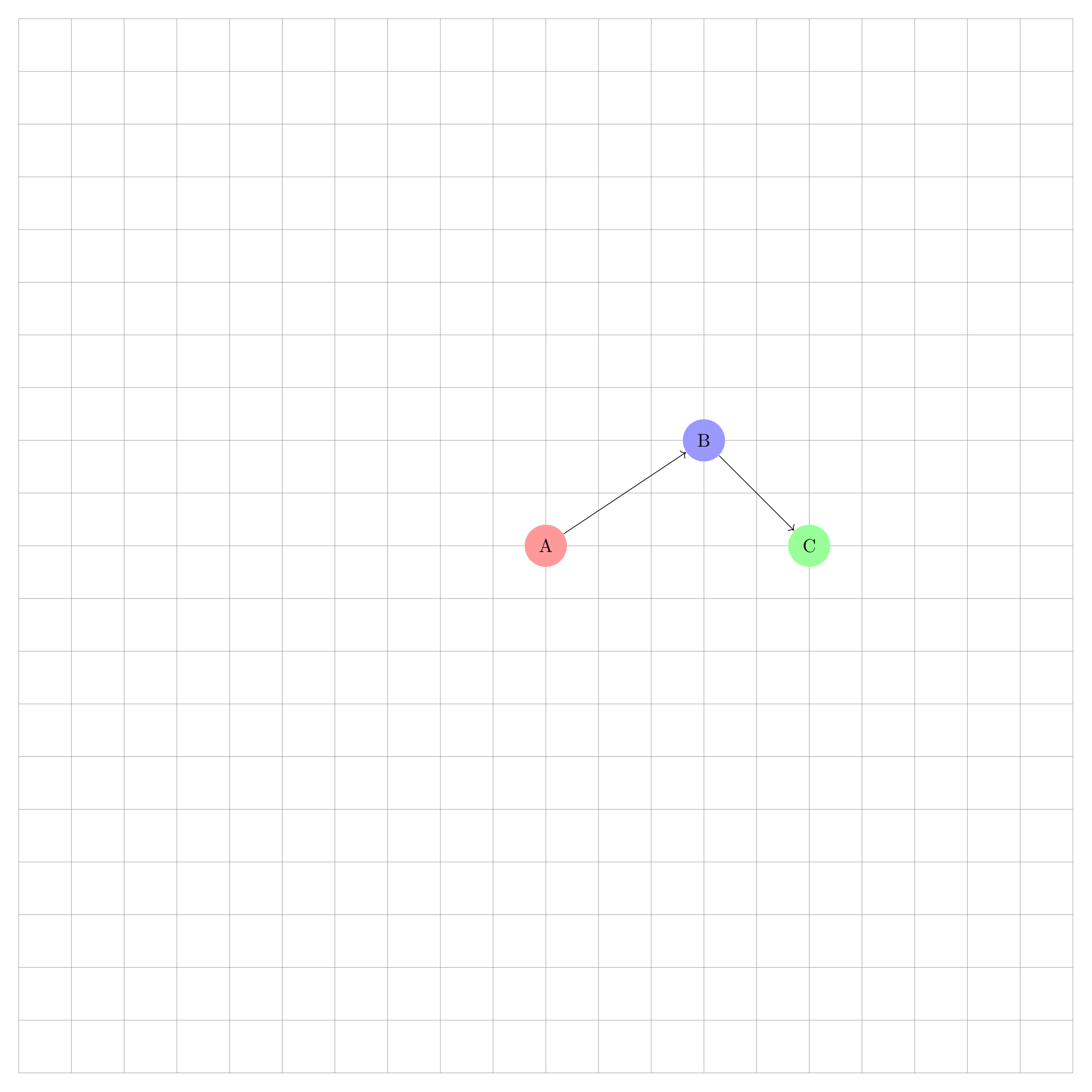
Show Tikz code
print(fig)% --------------------------------------------- %% Tikzfigure generated by tikzfigure v0.3.1 %% https://github.com/max-models/tikzfigure %% --------------------------------------------- %\begin{tikzpicture}[ axes/.style={}, important line/.style={very thick}, information text/.style={rounded corners, fill=red!10, inner sep=1ex} ] \draw[axes, ->, color=gray!70] (-1, 0) to (2, 0); \draw[axes, ->, color=gray!70] (0, -1) to (0, 2); \draw[important line, color=blue!70] (0, 0) to (1.2, 1.4); \node[information text, text width=3.2cm, anchor=west] (node0) at ({2.3}, {1.1}) {Named styles stay reusable};\end{tikzpicture}print(fig.generate_standalone())\documentclass[border=10pt]{standalone}\PassOptionsToPackage{dvipsnames,svgnames,x11names}{xcolor}\usepackage{tikz}\usepackage{pgfplots}\pgfplotsset{compat=newest}\usepgfplotslibrary{groupplots}\usetikzlibrary{arrows.meta}\begin{document}% --------------------------------------------- %% Tikzfigure generated by tikzfigure v0.3.1 %% https://github.com/max-models/tikzfigure %% --------------------------------------------- %\begin{tikzpicture}[ axes/.style={}, important line/.style={very thick}, information text/.style={rounded corners, fill=red!10, inner sep=1ex} ] \draw[axes, ->, color=gray!70] (-1, 0) to (2, 0); \draw[axes, ->, color=gray!70] (0, -1) to (0, 2); \draw[important line, color=blue!70] (0, 0) to (1.2, 1.4); \node[information text, text width=3.2cm, anchor=west] (node0) at ({2.3}, {1.1}) {Named styles stay reusable};\end{tikzpicture}
\end{document}scope(): local option blocks inside the figure
Section titled “scope(): local option blocks inside the figure”Use scope() when a style or transformation should only apply to part
of the figure. It wraps nested drawing commands in
\begin{scope}[...] ... \end{scope} with local options.
This is useful for small grouped coordinate systems, shifted sub-drawings, or temporary style changes that should not affect the rest of the figure.
fig = TikzFigure()
axes = fig.add_style("axes")
with fig.scope(options=[axes], xshift="0.5cm", yshift="0.3cm") as local:    local.draw([(-1, 0), (2, 0)], options=[arrows.forward], color="gray!70")    local.draw([(0, -1), (0, 2)], options=[arrows.forward], color="gray!70")
    A = local.node(        (0.8, 1.1),        label="A",        content="A",        shape="circle",        fill="blue!20",    )    B = local.node(        (1.6, 0.4),        label="B",        content="B",        shape="circle",        fill="orange!20",    )    local.draw(        [A, B],        options=[styles.thick],        color="purple!70",    )
fig.node(    (3.2, 1.2),    content="Outside the scope",    draw="none",    anchor="west",)
fig.show()
Show Tikz code
print(fig)% --------------------------------------------- %% Tikzfigure generated by tikzfigure v0.3.1 %% https://github.com/max-models/tikzfigure %% --------------------------------------------- %\begin{tikzpicture}[ axes/.style={} ] \begin{scope}[axes, xshift=0.5cm, yshift=0.3cm] \draw[->, color=gray!70] (-1, 0) to (2, 0); \draw[->, color=gray!70] (0, -1) to (0, 2); \node[shape=circle, fill=blue!20] (A) at ({0.8}, {1.1}) {A}; \node[shape=circle, fill=orange!20] (B) at ({1.6}, {0.4}) {B}; \draw[thick, color=purple!70] (A) to (B); \end{scope} \node[draw=none, anchor=west] (node0) at ({3.2}, {1.2}) {Outside the scope};\end{tikzpicture}print(fig.generate_standalone())\documentclass[border=10pt]{standalone}\PassOptionsToPackage{dvipsnames,svgnames,x11names}{xcolor}\usepackage{tikz}\usepackage{pgfplots}\pgfplotsset{compat=newest}\usepgfplotslibrary{groupplots}\usetikzlibrary{arrows.meta}\begin{document}% --------------------------------------------- %% Tikzfigure generated by tikzfigure v0.3.1 %% https://github.com/max-models/tikzfigure %% --------------------------------------------- %\begin{tikzpicture}[ axes/.style={} ] \begin{scope}[axes, xshift=0.5cm, yshift=0.3cm] \draw[->, color=gray!70] (-1, 0) to (2, 0); \draw[->, color=gray!70] (0, -1) to (0, 2); \node[shape=circle, fill=blue!20] (A) at ({0.8}, {1.1}) {A}; \node[shape=circle, fill=orange!20] (B) at ({1.6}, {0.4}) {B}; \draw[thick, color=purple!70] (A) to (B); \end{scope} \node[draw=none, anchor=west] (node0) at ({3.2}, {1.2}) {Outside the scope};\end{tikzpicture}
\end{document}grid: debug grid overlay
Section titled “grid: debug grid overlay”Pass grid=True to draw a background grid over the figure. This is a
handy positioning aid when you are still working out coordinates.
fig = TikzFigure(grid=True)
n1 = fig.node(    (0, 0),    shape="circle",    fill="red!40",    content="A",    minimum_size="0.8cm",)n2 = fig.node(    (3, 2),    shape="circle",    fill="blue!40",    content="B",    minimum_size="0.8cm",)n3 = fig.node(    (5, 0),    shape="circle",    fill="green!40",    content="C",    minimum_size="0.8cm",)fig.draw([n1, n2], arrows=arrows.forward)fig.draw([n2, n3], arrows=arrows.forward)
fig.show()
Show Tikz code
print(fig)% --------------------------------------------- %% Tikzfigure generated by tikzfigure v0.3.1 %% https://github.com/max-models/tikzfigure %% --------------------------------------------- %\begin{tikzpicture} \draw[step=1cm, gray, very thin] (-10,-10) grid (10,10); \node[shape=circle, fill=red!40, minimum size=0.8cm] (node0) at ({0}, {0}) {A}; \node[shape=circle, fill=blue!40, minimum size=0.8cm] (node1) at ({3}, {2}) {B}; \node[shape=circle, fill=green!40, minimum size=0.8cm] (node2) at ({5}, {0}) {C}; \draw[->] (node0) to (node1); \draw[->] (node1) to (node2);\end{tikzpicture}print(fig.generate_standalone())\documentclass[border=10pt]{standalone}\PassOptionsToPackage{dvipsnames,svgnames,x11names}{xcolor}\usepackage{tikz}\usepackage{pgfplots}\pgfplotsset{compat=newest}\usepgfplotslibrary{groupplots}\usetikzlibrary{arrows.meta}\begin{document}% --------------------------------------------- %% Tikzfigure generated by tikzfigure v0.3.1 %% https://github.com/max-models/tikzfigure %% --------------------------------------------- %\begin{tikzpicture} \draw[step=1cm, gray, very thin] (-10,-10) grid (10,10); \node[shape=circle, fill=red!40, minimum size=0.8cm] (node0) at ({0}, {0}) {A}; \node[shape=circle, fill=blue!40, minimum size=0.8cm] (node1) at ({3}, {2}) {B}; \node[shape=circle, fill=green!40, minimum size=0.8cm] (node2) at ({5}, {0}) {C}; \draw[->] (node0) to (node1); \draw[->] (node1) to (node2);\end{tikzpicture}
\end{document}The grid makes it easy to read off exact coordinates and spot
misalignments before removing grid=True for the final figure.
document_setup: raw LaTeX preamble additions
Section titled “document_setup: raw LaTeX preamble additions”document_setup is a raw LaTeX string inserted into the standalone
document preamble. It is the correct place for \usetikzlibrary{...}
calls and any other preamble additions that the figure needs.
A common use is loading the positioning library, which enables
relative placement keywords such as above_of, below_of, left_of,
right_of, and the node_distance parameter.
fig = TikzFigure(    document_setup=r"\usetikzlibrary{positioning}",)
root = fig.node(    (0, 0),    label="root",    content="Root",    shape="rectangle",    fill="purple!30",    minimum_size="1cm",)
# Relative positioning: omit x/y so no 'at (...)' is emittedfig.node(    label="above_node",    content="Above",    shape="rectangle",    fill="cyan!30",    minimum_size="1cm",    above_of="root",    node_distance="1.8cm",)
fig.node(    label="below_node",    content="Below",    shape="rectangle",    fill="cyan!30",    minimum_size="1cm",    below_of="root",    node_distance="1.8cm",)
fig.node(    label="left_node",    content="Left",    shape="rectangle",    fill="orange!30",    minimum_size="1cm",    left_of="root",    node_distance="2.5cm",)
fig.node(    label="right_node",    content="Right",    shape="rectangle",    fill="orange!30",    minimum_size="1cm",    right_of="root",    node_distance="2.5cm",)
for label in ["above_node", "below_node", "left_node", "right_node"]:    fig.draw(        ["root", label],        arrows=arrows.forward,        color="gray",    )
fig.show()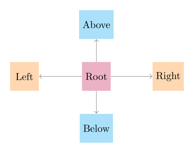
Show Tikz code
print(fig)% --------------------------------------------- %% Tikzfigure generated by tikzfigure v0.3.1 %% https://github.com/max-models/tikzfigure %% --------------------------------------------- %\begin{tikzpicture} \node[shape=rectangle, fill=purple!30, minimum size=1cm] (root) at ({0}, {0}) {Root}; \node[shape=rectangle, fill=cyan!30, minimum size=1cm, above of=root, node distance=1.8cm] (above_node) {Above}; \node[shape=rectangle, fill=cyan!30, minimum size=1cm, below of=root, node distance=1.8cm] (below_node) {Below}; \node[shape=rectangle, fill=orange!30, minimum size=1cm, left of=root, node distance=2.5cm] (left_node) {Left}; \node[shape=rectangle, fill=orange!30, minimum size=1cm, right of=root, node distance=2.5cm] (right_node) {Right}; \draw[->, color=gray] (root) to (above_node); \draw[->, color=gray] (root) to (below_node); \draw[->, color=gray] (root) to (left_node); \draw[->, color=gray] (root) to (right_node);\end{tikzpicture}print(fig.generate_standalone())\documentclass[border=10pt]{standalone}\PassOptionsToPackage{dvipsnames,svgnames,x11names}{xcolor}\usepackage{tikz}\usepackage{pgfplots}\pgfplotsset{compat=newest}\usepgfplotslibrary{groupplots}\usetikzlibrary{arrows.meta}% Custom document setup\usetikzlibrary{positioning}\begin{document}% --------------------------------------------- %% Tikzfigure generated by tikzfigure v0.3.1 %% https://github.com/max-models/tikzfigure %% --------------------------------------------- %\begin{tikzpicture} \node[shape=rectangle, fill=purple!30, minimum size=1cm] (root) at ({0}, {0}) {Root}; \node[shape=rectangle, fill=cyan!30, minimum size=1cm, above of=root, node distance=1.8cm] (above_node) {Above}; \node[shape=rectangle, fill=cyan!30, minimum size=1cm, below of=root, node distance=1.8cm] (below_node) {Below}; \node[shape=rectangle, fill=orange!30, minimum size=1cm, left of=root, node distance=2.5cm] (left_node) {Left}; \node[shape=rectangle, fill=orange!30, minimum size=1cm, right of=root, node distance=2.5cm] (right_node) {Right}; \draw[->, color=gray] (root) to (above_node); \draw[->, color=gray] (root) to (below_node); \draw[->, color=gray] (root) to (left_node); \draw[->, color=gray] (root) to (right_node);\end{tikzpicture}
\end{document}add_package(): additional LaTeX packages
Section titled “add_package(): additional LaTeX packages”Call add_package() for each package you want in the standalone
preamble. Each package name becomes a \usepackage{name} line in the
standalone preamble. This is useful when your figure content uses macros
from packages like amsmath or xcolor.
fig = TikzFigure()fig.add_package("amsmath")fig.add_package("xcolor")
# amsmath lets us use \dfrac inside node contentfig.node(    (0, 2),    content=r"$\dfrac{a}{b} + \sqrt{c}$",    shape="rectangle",    fill="yellow!20",    draw="orange",    minimum_width="3cm",    minimum_height="1.2cm",)
fig.node(    (0, 0),    content=r"$\sum_{k=1}^{n} k = \dfrac{n(n+1)}{2}$",    shape="rectangle",    fill="green!20",    draw="teal",    minimum_width="4cm",    minimum_height="1.2cm",)
fig.show()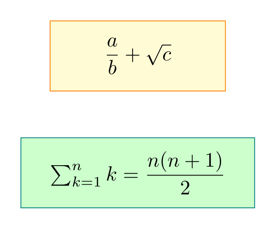
Show Tikz code
print(fig)% --------------------------------------------- %% Tikzfigure generated by tikzfigure v0.3.1 %% https://github.com/max-models/tikzfigure %% --------------------------------------------- %\begin{tikzpicture} \node[shape=rectangle, fill=yellow!20, draw=orange, minimum width=3cm, minimum height=1.2cm] (node0) at ({0}, {2}) {$\dfrac{a}{b} + \sqrt{c}$}; \node[shape=rectangle, fill=green!20, draw=teal, minimum width=4cm, minimum height=1.2cm] (node1) at ({0}, {0}) {$\sum_{k=1}^{n} k = \dfrac{n(n+1)}{2}$};\end{tikzpicture}print(fig.generate_standalone())\documentclass[border=10pt]{standalone}\PassOptionsToPackage{dvipsnames,svgnames,x11names}{xcolor}\usepackage{tikz}\usepackage{pgfplots}\pgfplotsset{compat=newest}\usepgfplotslibrary{groupplots}\usetikzlibrary{arrows.meta}\usepackage{amsmath}\usepackage{xcolor}\begin{document}% --------------------------------------------- %% Tikzfigure generated by tikzfigure v0.3.1 %% https://github.com/max-models/tikzfigure %% --------------------------------------------- %\begin{tikzpicture} \node[shape=rectangle, fill=yellow!20, draw=orange, minimum width=3cm, minimum height=1.2cm] (node0) at ({0}, {2}) {$\dfrac{a}{b} + \sqrt{c}$}; \node[shape=rectangle, fill=green!20, draw=teal, minimum width=4cm, minimum height=1.2cm] (node1) at ({0}, {0}) {$\sum_{k=1}^{n} k = \dfrac{n(n+1)}{2}$};\end{tikzpicture}
\end{document}generate_standalone(): inspecting the full document
Section titled “generate_standalone(): inspecting the full document”generate_standalone() returns a complete compilable LaTeX document
including the preamble. This shows exactly how document_setup,
add_package(), and usetikzlibrary() are woven into the output.
fig = TikzFigure()fig.add_package("amsmath")fig.usetikzlibrary("positioning")
fig.node(    (0, 0),    content="Hello",    shape="circle",    fill="blue!30",)
print(fig.generate_standalone())\documentclass[border=10pt]{standalone}\PassOptionsToPackage{dvipsnames,svgnames,x11names}{xcolor}\usepackage{tikz}\usepackage{pgfplots}\pgfplotsset{compat=newest}\usepgfplotslibrary{groupplots}\usetikzlibrary{arrows.meta,positioning}\usepackage{amsmath}\begin{document}% --------------------------------------------- %% Tikzfigure generated by tikzfigure v0.3.1 %% https://github.com/max-models/tikzfigure %% --------------------------------------------- %\begin{tikzpicture} \node[shape=circle, fill=blue!30] (node0) at ({0}, {0}) {Hello};\end{tikzpicture}
\end{document}Show Tikz code
print(fig)% --------------------------------------------- %% Tikzfigure generated by tikzfigure v0.3.1 %% https://github.com/max-models/tikzfigure %% --------------------------------------------- %\begin{tikzpicture} \node[shape=circle, fill=blue!30] (node0) at ({0}, {0}) {Hello};\end{tikzpicture}print(fig.generate_standalone())\documentclass[border=10pt]{standalone}\PassOptionsToPackage{dvipsnames,svgnames,x11names}{xcolor}\usepackage{tikz}\usepackage{pgfplots}\pgfplotsset{compat=newest}\usepgfplotslibrary{groupplots}\usetikzlibrary{arrows.meta,positioning}\usepackage{amsmath}\begin{document}% --------------------------------------------- %% Tikzfigure generated by tikzfigure v0.3.1 %% https://github.com/max-models/tikzfigure %% --------------------------------------------- %\begin{tikzpicture} \node[shape=circle, fill=blue!30] (node0) at ({0}, {0}) {Hello};\end{tikzpicture}
\end{document}label: wrapping in a figure environment
Section titled “label: wrapping in a figure environment”When label is set, tikzfigure wraps the tikzpicture in a
\begin{figure}...\end{figure} environment and adds \label{...} for
cross-referencing.
fig = TikzFigure(    label="fig:simple-graph",)
A = fig.node(    (0, 1),    label="A",    content="A",    shape="circle",    fill="cyan!40",)B = fig.node(    (3, 1),    label="B",    content="B",    shape="circle",    fill="cyan!40",)C = fig.node(    (1.5, -1),    label="C",    content="C",    shape="circle",    fill="cyan!40",)
fig.draw([A, B], arrows=arrows.forward)fig.draw([A, C], arrows=arrows.forward)fig.draw([B, C], arrows=arrows.forward)
print(fig.generate_tikz())\begin{figure} % --------------------------------------------- % % Tikzfigure generated by tikzfigure v0.3.1 % % https://github.com/max-models/tikzfigure % % --------------------------------------------- % \begin{tikzpicture} \node[shape=circle, fill=cyan!40] (A) at ({0}, {1}) {A}; \node[shape=circle, fill=cyan!40] (B) at ({3}, {1}) {B}; \node[shape=circle, fill=cyan!40] (C) at ({1.5}, {-1}) {C}; \draw[->] (A) to (B); \draw[->] (A) to (C); \draw[->] (B) to (C); \end{tikzpicture} \label{fig:simple-graph}\end{figure}Show Tikz code
print(fig)\begin{figure} % --------------------------------------------- % % Tikzfigure generated by tikzfigure v0.3.1 % % https://github.com/max-models/tikzfigure % % --------------------------------------------- % \begin{tikzpicture} \node[shape=circle, fill=cyan!40] (A) at ({0}, {1}) {A}; \node[shape=circle, fill=cyan!40] (B) at ({3}, {1}) {B}; \node[shape=circle, fill=cyan!40] (C) at ({1.5}, {-1}) {C}; \draw[->] (A) to (B); \draw[->] (A) to (C); \draw[->] (B) to (C); \end{tikzpicture} \label{fig:simple-graph}\end{figure}print(fig.generate_standalone())\documentclass[border=10pt]{standalone}\PassOptionsToPackage{dvipsnames,svgnames,x11names}{xcolor}\usepackage{tikz}\usepackage{pgfplots}\pgfplotsset{compat=newest}\usepgfplotslibrary{groupplots}\usetikzlibrary{arrows.meta}\begin{document}\begin{figure} % --------------------------------------------- % % Tikzfigure generated by tikzfigure v0.3.1 % % https://github.com/max-models/tikzfigure % % --------------------------------------------- % \begin{tikzpicture} \node[shape=circle, fill=cyan!40] (A) at ({0}, {1}) {A}; \node[shape=circle, fill=cyan!40] (B) at ({3}, {1}) {B}; \node[shape=circle, fill=cyan!40] (C) at ({1.5}, {-1}) {C}; \draw[->] (A) to (B); \draw[->] (A) to (C); \draw[->] (B) to (C); \end{tikzpicture} \label{fig:simple-graph}\end{figure}
\end{document}Notice that generate_tikz() now includes the \begin{figure} wrapper.
figsize: Jupyter display-size hint
Section titled “figsize: Jupyter display-size hint”figsize=(width, height) controls how large the compiled image appears
in Jupyter. It is purely a display hint — it does not affect the LaTeX
output or the saved file.
fig = TikzFigure(figsize=(4, 2))
fig.node(    (0, 0),    shape="circle",    fill="red!40",    content="Small",    minimum_size="1.5cm",)fig.node(    (3, 0),    shape="circle",    fill="blue!40",    content="display",    minimum_size="1.5cm",)
fig.show()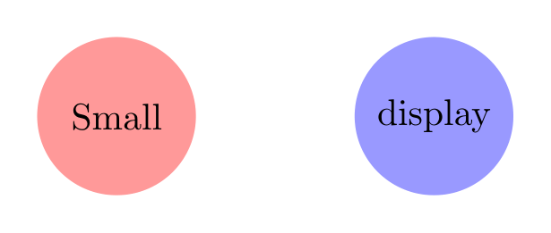
Show Tikz code
print(fig)% --------------------------------------------- %% Tikzfigure generated by tikzfigure v0.3.1 %% https://github.com/max-models/tikzfigure %% --------------------------------------------- %\begin{tikzpicture} \node[shape=circle, fill=red!40, minimum size=1.5cm] (node0) at ({0}, {0}) {Small}; \node[shape=circle, fill=blue!40, minimum size=1.5cm] (node1) at ({3}, {0}) {display};\end{tikzpicture}print(fig.generate_standalone())\documentclass[border=10pt]{standalone}\PassOptionsToPackage{dvipsnames,svgnames,x11names}{xcolor}\usepackage{tikz}\usepackage{pgfplots}\pgfplotsset{compat=newest}\usepgfplotslibrary{groupplots}\usetikzlibrary{arrows.meta}\begin{document}% --------------------------------------------- %% Tikzfigure generated by tikzfigure v0.3.1 %% https://github.com/max-models/tikzfigure %% --------------------------------------------- %\begin{tikzpicture} \node[shape=circle, fill=red!40, minimum size=1.5cm] (node0) at ({0}, {0}) {Small}; \node[shape=circle, fill=blue!40, minimum size=1.5cm] (node1) at ({3}, {0}) {display};\end{tikzpicture}
\end{document}# Same figure, larger display sizefig = TikzFigure(figsize=(8, 4))
fig.node( (0, 0), shape="circle", fill="red!40", content="Large", minimum_size="1.5cm",)fig.node( (3, 0), shape="circle", fill="blue!40", content="display", minimum_size="1.5cm",)
fig.show()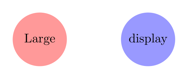
Show Tikz code
print(fig)% --------------------------------------------- %% Tikzfigure generated by tikzfigure v0.3.1 %% https://github.com/max-models/tikzfigure %% --------------------------------------------- %\begin{tikzpicture} \node[shape=circle, fill=red!40, minimum size=1.5cm] (node0) at ({0}, {0}) {Large}; \node[shape=circle, fill=blue!40, minimum size=1.5cm] (node1) at ({3}, {0}) {display};\end{tikzpicture}print(fig.generate_standalone())\documentclass[border=10pt]{standalone}\PassOptionsToPackage{dvipsnames,svgnames,x11names}{xcolor}\usepackage{tikz}\usepackage{pgfplots}\pgfplotsset{compat=newest}\usepgfplotslibrary{groupplots}\usetikzlibrary{arrows.meta}\begin{document}% --------------------------------------------- %% Tikzfigure generated by tikzfigure v0.3.1 %% https://github.com/max-models/tikzfigure %% --------------------------------------------- %\begin{tikzpicture} \node[shape=circle, fill=red!40, minimum size=1.5cm] (node0) at ({0}, {0}) {Large}; \node[shape=circle, fill=blue!40, minimum size=1.5cm] (node1) at ({3}, {0}) {display};\end{tikzpicture}
\end{document}The LaTeX code for both figures is identical — only the rendered size in the notebook differs.