2D Plots: Styling
Customize plot appearance with colors, markers, line styles, and custom ticks.
from tikzfigure import TikzFigure, marks, stylesColors and markers
Section titled “Colors and markers”pgfplots supports named colors and various marker types:
fig = TikzFigure()
ax = fig.axis2d(    xlabel="Month",    ylabel="Temperature",    xlim=(0, 13),    grid=True,)
months = [1, 2, 3, 4, 5, 6, 7, 8, 9, 10, 11, 12]temp_seattle = [-5, -4, 0, 5, 10, 15, 18, 17, 12, 6, 0, -4]temp_phoenix = [12, 15, 18, 24, 30, 36, 38, 37, 33, 26, 18, 12]
ax.add_plot(    months,    temp_seattle,    label="Seattle",    color="blue",    mark=marks.circle,)ax.add_plot(    months,    temp_phoenix,    label="Phoenix",    color="red",    mark=marks.square,)
ax.set_legend(position="north west")fig.show()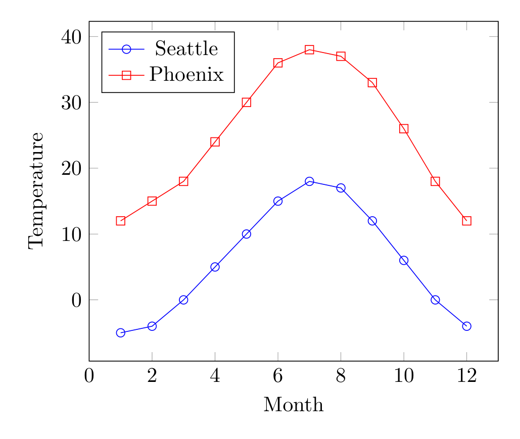
Show Tikz code
print(fig)% --------------------------------------------- %% Tikzfigure generated by tikzfigure v0.3.1 %% https://github.com/max-models/tikzfigure %% --------------------------------------------- %\begin{tikzpicture} \begin{axis}[xlabel=Month, ylabel=Temperature, xmin=0, xmax=13, grid=major, legend pos=north west] \addplot[color=blue, mark=o] coordinates {(1,-5) (2,-4) (3,0) (4,5) (5,10) (6,15) (7,18) (8,17) (9,12) (10,6) (11,0) (12,-4)}; \addplot[color=red, mark=square] coordinates {(1,12) (2,15) (3,18) (4,24) (5,30) (6,36) (7,38) (8,37) (9,33) (10,26) (11,18) (12,12)}; \legend{Seattle, Phoenix} \end{axis}\end{tikzpicture}print(fig.generate_standalone())\documentclass[border=10pt]{standalone}\PassOptionsToPackage{dvipsnames,svgnames,x11names}{xcolor}\usepackage{tikz}\usepackage{pgfplots}\pgfplotsset{compat=newest}\usepgfplotslibrary{groupplots}\usetikzlibrary{arrows.meta}\usepackage{pgfplots}\begin{document}% --------------------------------------------- %% Tikzfigure generated by tikzfigure v0.3.1 %% https://github.com/max-models/tikzfigure %% --------------------------------------------- %\begin{tikzpicture} \begin{axis}[xlabel=Month, ylabel=Temperature, xmin=0, xmax=13, grid=major, legend pos=north west] \addplot[color=blue, mark=o] coordinates {(1,-5) (2,-4) (3,0) (4,5) (5,10) (6,15) (7,18) (8,17) (9,12) (10,6) (11,0) (12,-4)}; \addplot[color=red, mark=square] coordinates {(1,12) (2,15) (3,18) (4,24) (5,30) (6,36) (7,38) (8,37) (9,33) (10,26) (11,18) (12,12)}; \legend{Seattle, Phoenix} \end{axis}\end{tikzpicture}
\end{document}Available markers: raw strings still work, and so do objects like
marks.circle, marks.asterisk, marks.square, marks.triangle,
marks.diamond, marks.x, and marks.plus
Available colors: red, blue, green, black, plus mixing like
blue!50!red
Line styles and thickness
Section titled “Line styles and thickness”Customize line appearance with options and line_width:
fig = TikzFigure()
ax = fig.axis2d(    xlabel="$X$",    ylabel="$Y$",    xlim=(0, 10),    grid=True,)
x = [0, 1, 2, 3, 4, 5, 6, 7, 8, 9, 10]y1 = [0, 1, 4, 9, 16, 25, 36, 49, 64, 81, 100]y2 = [0, 2, 4, 6, 8, 10, 12, 14, 16, 18, 20]
ax.add_plot(    x,    y1,    label="Thick solid",    color="red",    line_width="2pt",)ax.add_plot(    x,    y2,    label="Thin dashed",    color="blue",    options=[styles.dashed],)
ax.set_legend()fig.show()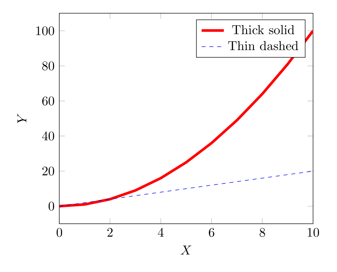
Show Tikz code
print(fig)% --------------------------------------------- %% Tikzfigure generated by tikzfigure v0.3.1 %% https://github.com/max-models/tikzfigure %% --------------------------------------------- %\begin{tikzpicture} \begin{axis}[xlabel=$X$, ylabel=$Y$, xmin=0, xmax=10, grid=major, legend pos=north east] \addplot[color=red, line width=2pt] coordinates {(0,0) (1,1) (2,4) (3,9) (4,16) (5,25) (6,36) (7,49) (8,64) (9,81) (10,100)}; \addplot[dashed, color=blue] coordinates {(0,0) (1,2) (2,4) (3,6) (4,8) (5,10) (6,12) (7,14) (8,16) (9,18) (10,20)}; \legend{Thick solid, Thin dashed} \end{axis}\end{tikzpicture}print(fig.generate_standalone())\documentclass[border=10pt]{standalone}\PassOptionsToPackage{dvipsnames,svgnames,x11names}{xcolor}\usepackage{tikz}\usepackage{pgfplots}\pgfplotsset{compat=newest}\usepgfplotslibrary{groupplots}\usetikzlibrary{arrows.meta}\usepackage{pgfplots}\begin{document}% --------------------------------------------- %% Tikzfigure generated by tikzfigure v0.3.1 %% https://github.com/max-models/tikzfigure %% --------------------------------------------- %\begin{tikzpicture} \begin{axis}[xlabel=$X$, ylabel=$Y$, xmin=0, xmax=10, grid=major, legend pos=north east] \addplot[color=red, line width=2pt] coordinates {(0,0) (1,1) (2,4) (3,9) (4,16) (5,25) (6,36) (7,49) (8,64) (9,81) (10,100)}; \addplot[dashed, color=blue] coordinates {(0,0) (1,2) (2,4) (3,6) (4,8) (5,10) (6,12) (7,14) (8,16) (9,18) (10,20)}; \legend{Thick solid, Thin dashed} \end{axis}\end{tikzpicture}
\end{document}options accepts pgfplots flags: "dashed", "dotted",
"densely dashed", "only marks".
Custom ticks and labels
Section titled “Custom ticks and labels”Control tick positions and labels:
fig = TikzFigure()
ax = fig.axis2d(    xlabel="Grade",    ylabel="Count",    xlim=(0.5, 4.5),    ylim=(0, 30),)
ax.add_plot(    [1, 2, 3, 4],    [5, 12, 18, 10],    label="Students",    color="green",    mark="*",)
# Custom x-axis labelsax.set_ticks(    "x",    [1, 2, 3, 4],    labels=["A", "B", "C", "D"],)
# Y-axis ticks at multiples of 5ax.set_ticks("y", [0, 5, 10, 15, 20, 25, 30])
ax.set_legend()fig.show()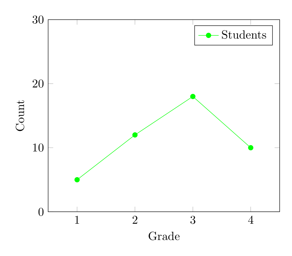
Show Tikz code
print(fig)% --------------------------------------------- %% Tikzfigure generated by tikzfigure v0.3.1 %% https://github.com/max-models/tikzfigure %% --------------------------------------------- %\begin{tikzpicture} \begin{axis}[xlabel=Grade, ylabel=Count, xmin=0.5, xmax=4.5, ymin=0, ymax=30, grid=major, legend pos=north east] \addplot[color=green, mark=*] coordinates {(1,5) (2,12) (3,18) (4,10)}; \legend{Students} \end{axis}\end{tikzpicture}print(fig.generate_standalone())\documentclass[border=10pt]{standalone}\PassOptionsToPackage{dvipsnames,svgnames,x11names}{xcolor}\usepackage{tikz}\usepackage{pgfplots}\pgfplotsset{compat=newest}\usepgfplotslibrary{groupplots}\usetikzlibrary{arrows.meta}\usepackage{pgfplots}\begin{document}% --------------------------------------------- %% Tikzfigure generated by tikzfigure v0.3.1 %% https://github.com/max-models/tikzfigure %% --------------------------------------------- %\begin{tikzpicture} \begin{axis}[xlabel=Grade, ylabel=Count, xmin=0.5, xmax=4.5, ymin=0, ymax=30, grid=major, legend pos=north east] \addplot[color=green, mark=*] coordinates {(1,5) (2,12) (3,18) (4,10)}; \legend{Students} \end{axis}\end{tikzpicture}
\end{document}Scatter plots (only marks)
Section titled “Scatter plots (only marks)”Use options=["only marks"] to show only markers without connecting
lines:
fig = TikzFigure()
ax = fig.axis2d(    xlabel="X",    ylabel="Y",    xlim=(-1, 5),    ylim=(-2, 10),    grid=True,)
# Noisy data pointsx_data = [0, 1, 1.5, 2, 2.5, 3, 4]y_data = [0, 0.9, 2.2, 3.8, 4.5, 6.2, 8.1]
# Fitted linex_fit = [i * 0.1 for i in range(50)]y_fit = [2 * x + 0.5 for x in x_fit]
ax.add_plot(    x_data,    y_data,    label="Data",    color="red",    mark="o",    mark_size="2pt",    options=["only marks"],)ax.add_plot(    x_fit,    y_fit,    label="Fit: y = 2x + 0.5",    color="blue",)
ax.set_legend(position="north west")fig.show()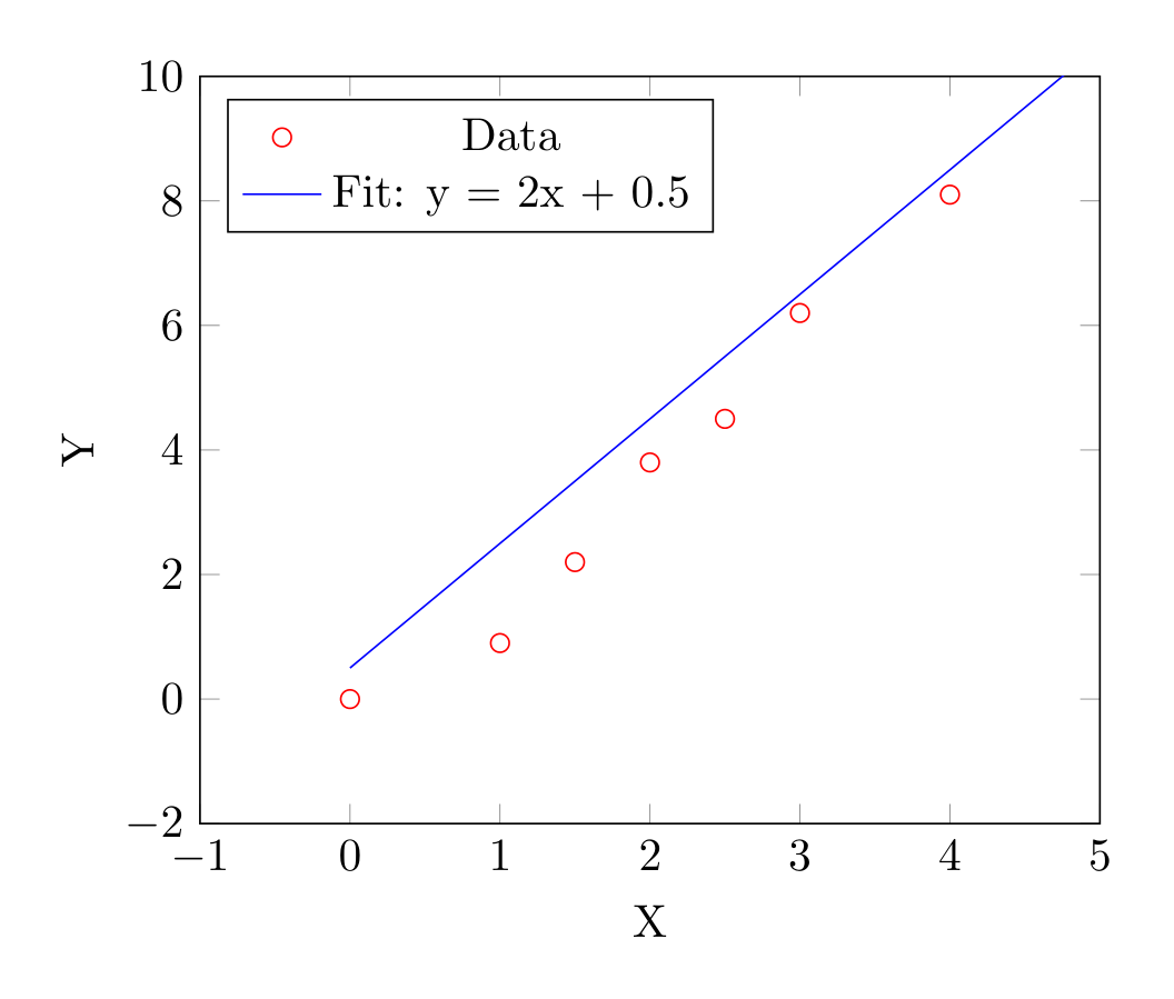
Show Tikz code
print(fig)% --------------------------------------------- %% Tikzfigure generated by tikzfigure v0.3.1 %% https://github.com/max-models/tikzfigure %% --------------------------------------------- %\begin{tikzpicture} \begin{axis}[xlabel=X, ylabel=Y, xmin=-1, xmax=5, ymin=-2, ymax=10, grid=major, legend pos=north west] \addplot[only marks, color=red, mark=o, mark size=2pt] coordinates {(0,0) (1,0.9) (1.5,2.2) (2,3.8) (2.5,4.5) (3,6.2) (4,8.1)}; \addplot[color=blue] coordinates {(0.0,0.5) (0.1,0.7) (0.2,0.9) (0.30000000000000004,1.1) (0.4,1.3) (0.5,1.5) (0.6000000000000001,1.7000000000000002) (0.7000000000000001,1.9000000000000001) (0.8,2.1) (0.9,2.3) (1.0,2.5) (1.1,2.7) (1.2000000000000002,2.9000000000000004) (1.3,3.1) (1.4000000000000001,3.3000000000000003) (1.5,3.5) (1.6,3.7) (1.7000000000000002,3.9000000000000004) (1.8,4.1) (1.9000000000000001,4.300000000000001) (2.0,4.5) (2.1,4.7) (2.2,4.9) (2.3000000000000003,5.1000000000000005) (2.4000000000000004,5.300000000000001) (2.5,5.5) (2.6,5.7) (2.7,5.9) (2.8000000000000003,6.1000000000000005) (2.9000000000000004,6.300000000000001) (3.0,6.5) (3.1,6.7) (3.2,6.9) (3.3000000000000003,7.1000000000000005) (3.4000000000000004,7.300000000000001) (3.5,7.5) (3.6,7.7) (3.7,7.9) (3.8000000000000003,8.100000000000001) (3.9000000000000004,8.3) (4.0,8.5) (4.1000000000000005,8.700000000000001) (4.2,8.9) (4.3,9.1) (4.4,9.3) (4.5,9.5) (4.6000000000000005,9.700000000000001) (4.7,9.9) (4.800000000000001,10.100000000000001) (4.9,10.3)}; \legend{Data, Fit: y = 2x + 0.5} \end{axis}\end{tikzpicture}print(fig.generate_standalone())\documentclass[border=10pt]{standalone}\PassOptionsToPackage{dvipsnames,svgnames,x11names}{xcolor}\usepackage{tikz}\usepackage{pgfplots}\pgfplotsset{compat=newest}\usepgfplotslibrary{groupplots}\usetikzlibrary{arrows.meta}\usepackage{pgfplots}\begin{document}% --------------------------------------------- %% Tikzfigure generated by tikzfigure v0.3.1 %% https://github.com/max-models/tikzfigure %% --------------------------------------------- %\begin{tikzpicture} \begin{axis}[xlabel=X, ylabel=Y, xmin=-1, xmax=5, ymin=-2, ymax=10, grid=major, legend pos=north west] \addplot[only marks, color=red, mark=o, mark size=2pt] coordinates {(0,0) (1,0.9) (1.5,2.2) (2,3.8) (2.5,4.5) (3,6.2) (4,8.1)}; \addplot[color=blue] coordinates {(0.0,0.5) (0.1,0.7) (0.2,0.9) (0.30000000000000004,1.1) (0.4,1.3) (0.5,1.5) (0.6000000000000001,1.7000000000000002) (0.7000000000000001,1.9000000000000001) (0.8,2.1) (0.9,2.3) (1.0,2.5) (1.1,2.7) (1.2000000000000002,2.9000000000000004) (1.3,3.1) (1.4000000000000001,3.3000000000000003) (1.5,3.5) (1.6,3.7) (1.7000000000000002,3.9000000000000004) (1.8,4.1) (1.9000000000000001,4.300000000000001) (2.0,4.5) (2.1,4.7) (2.2,4.9) (2.3000000000000003,5.1000000000000005) (2.4000000000000004,5.300000000000001) (2.5,5.5) (2.6,5.7) (2.7,5.9) (2.8000000000000003,6.1000000000000005) (2.9000000000000004,6.300000000000001) (3.0,6.5) (3.1,6.7) (3.2,6.9) (3.3000000000000003,7.1000000000000005) (3.4000000000000004,7.300000000000001) (3.5,7.5) (3.6,7.7) (3.7,7.9) (3.8000000000000003,8.100000000000001) (3.9000000000000004,8.3) (4.0,8.5) (4.1000000000000005,8.700000000000001) (4.2,8.9) (4.3,9.1) (4.4,9.3) (4.5,9.5) (4.6000000000000005,9.700000000000001) (4.7,9.9) (4.800000000000001,10.100000000000001) (4.9,10.3)}; \legend{Data, Fit: y = 2x + 0.5} \end{axis}\end{tikzpicture}
\end{document}Axes on different layers
Section titled “Axes on different layers”Axes can be assigned to layers to control stacking with other TikZ elements:
fig = TikzFigure()
ax = fig.axis2d(    xlabel="X",    ylabel="Y",    xlim=(0, 5),    ylim=(0, 5),    layer=1,)ax.add_plot(    [0, 1, 2, 3, 4, 5],    [0, 1, 2, 3, 4, 5],    label="data",    color="red",)ax.set_legend(position="north west")
# Background shape on layer 0fig.node(    (2.5, 2.5),    label="bg",    content="Background",    shape="circle",    minimum_size="4cm",    fill="gray!20",    draw="none",    layer=0,)
# Foreground annotation on layer 2fig.node(    (4, 4),    label="fg",    content="Foreground!",    shape="rectangle",    fill="yellow!30",    layer=2,)
fig.show()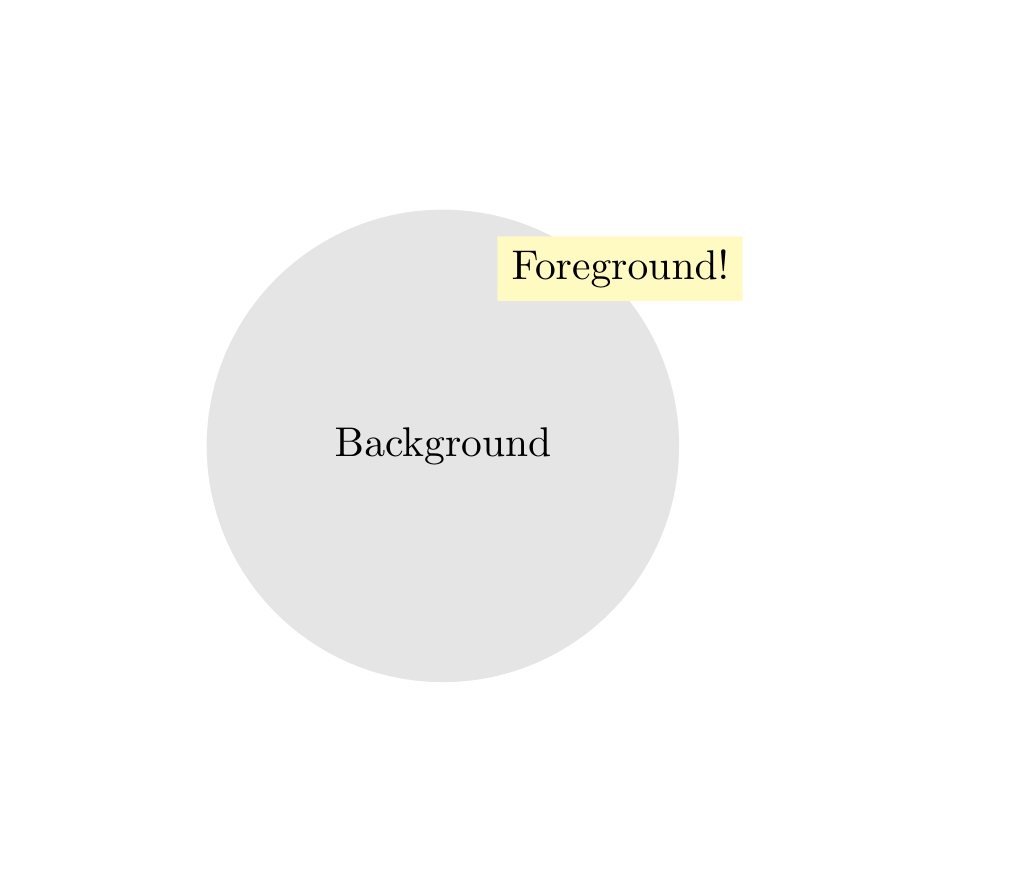
Show Tikz code
print(fig)% --------------------------------------------- %% Tikzfigure generated by tikzfigure v0.3.1 %% https://github.com/max-models/tikzfigure %% --------------------------------------------- %\begin{tikzpicture} % Define the layers library \pgfdeclarelayer{0} \pgfdeclarelayer{1} \pgfdeclarelayer{2} \pgfsetlayers{0,1,2}
% Layer 0 \begin{pgfonlayer}{0} \node[shape=circle, fill=gray!20, draw=none, minimum size=4cm] (bg) at ({2.5}, {2.5}) {Background}; \end{pgfonlayer}{0}
% Layer 2 \begin{pgfonlayer}{2} \node[shape=rectangle, fill=yellow!30] (fg) at ({4}, {4}) {Foreground!}; \end{pgfonlayer}{2}
% Layer 1 \begin{pgfonlayer}{1} \begin{axis}[xlabel=X, ylabel=Y, xmin=0, xmax=5, ymin=0, ymax=5, grid=major, legend pos=north west] \addplot[color=red] coordinates {(0,0) (1,1) (2,2) (3,3) (4,4) (5,5)}; \legend{data} \end{axis} \end{pgfonlayer}{1}\end{tikzpicture}print(fig.generate_standalone())\documentclass[border=10pt]{standalone}\PassOptionsToPackage{dvipsnames,svgnames,x11names}{xcolor}\usepackage{tikz}\usepackage{pgfplots}\pgfplotsset{compat=newest}\usepgfplotslibrary{groupplots}\usetikzlibrary{arrows.meta}\usepackage{pgfplots}\begin{document}% --------------------------------------------- %% Tikzfigure generated by tikzfigure v0.3.1 %% https://github.com/max-models/tikzfigure %% --------------------------------------------- %\begin{tikzpicture} % Define the layers library \pgfdeclarelayer{0} \pgfdeclarelayer{1} \pgfdeclarelayer{2} \pgfsetlayers{0,1,2}
% Layer 0 \begin{pgfonlayer}{0} \node[shape=circle, fill=gray!20, draw=none, minimum size=4cm] (bg) at ({2.5}, {2.5}) {Background}; \end{pgfonlayer}{0}
% Layer 2 \begin{pgfonlayer}{2} \node[shape=rectangle, fill=yellow!30] (fg) at ({4}, {4}) {Foreground!}; \end{pgfonlayer}{2}
% Layer 1 \begin{pgfonlayer}{1} \begin{axis}[xlabel=X, ylabel=Y, xmin=0, xmax=5, ymin=0, ymax=5, grid=major, legend pos=north west] \addplot[color=red] coordinates {(0,0) (1,1) (2,2) (3,3) (4,4) (5,5)}; \legend{data} \end{axis} \end{pgfonlayer}{1}\end{tikzpicture}
\end{document}