Loops
Repetitive structures — grids, chains, matrices of nodes — can be
created in two ways: with Python loops that call node / draw
many times, or with native TikZ \foreach loops via fig.loop(),
which embeds the loop directly in the generated LaTeX instead of
unrolling it in Python.
Benefits of TikZ \foreach loops: - the generated .tex file is much
shorter and more readable - loop variable values are available as TikZ
expressions (e.g. \i) at compile time - loops can be nested
This tutorial covers: - Python loop vs TikZ \foreach — side-by-side
comparison - basic loop usage - loop variable in colour expressions -
nested loops for a grid - variable for reusable TikZ constants - a
practical chain-of-boxes diagram
from tikzfigure import TikzFigure, arrowsPython loop vs TikZ \foreach — a side-by-side comparison
Section titled “Python loop vs TikZ \foreach — a side-by-side comparison”Both approaches produce the same visual output: a row of five circles.
The key difference is in the generated LaTeX. The Python loop unrolls
every node into a separate \node command, while loop emits a single
compact \foreach block.
Python loop version:
fig = TikzFigure()
for i in range(5):    fig.node(        (i * 2, 0),        shape="circle",        fill="blue!40",        content=str(i),        minimum_size="0.8cm",    )
fig.show()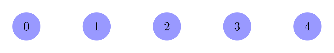
Show Tikz code
print(fig)% --------------------------------------------- %% Tikzfigure generated by tikzfigure v0.3.1 %% https://github.com/max-models/tikzfigure %% --------------------------------------------- %\begin{tikzpicture} \node[shape=circle, fill=blue!40, minimum size=0.8cm] (node0) at ({0}, {0}) {0}; \node[shape=circle, fill=blue!40, minimum size=0.8cm] (node1) at ({2}, {0}) {1}; \node[shape=circle, fill=blue!40, minimum size=0.8cm] (node2) at ({4}, {0}) {2}; \node[shape=circle, fill=blue!40, minimum size=0.8cm] (node3) at ({6}, {0}) {3}; \node[shape=circle, fill=blue!40, minimum size=0.8cm] (node4) at ({8}, {0}) {4};\end{tikzpicture}print(fig.generate_standalone())\documentclass[border=10pt]{standalone}\PassOptionsToPackage{dvipsnames,svgnames,x11names}{xcolor}\usepackage{tikz}\usepackage{pgfplots}\pgfplotsset{compat=newest}\usepgfplotslibrary{groupplots}\usetikzlibrary{arrows.meta}\begin{document}% --------------------------------------------- %% Tikzfigure generated by tikzfigure v0.3.1 %% https://github.com/max-models/tikzfigure %% --------------------------------------------- %\begin{tikzpicture} \node[shape=circle, fill=blue!40, minimum size=0.8cm] (node0) at ({0}, {0}) {0}; \node[shape=circle, fill=blue!40, minimum size=0.8cm] (node1) at ({2}, {0}) {1}; \node[shape=circle, fill=blue!40, minimum size=0.8cm] (node2) at ({4}, {0}) {2}; \node[shape=circle, fill=blue!40, minimum size=0.8cm] (node3) at ({6}, {0}) {3}; \node[shape=circle, fill=blue!40, minimum size=0.8cm] (node4) at ({8}, {0}) {4};\end{tikzpicture}
\end{document}TikZ \foreach version — same output, much shorter LaTeX:
fig = TikzFigure()
with fig.loop(    "i",    range(5),    comment="Row of circles",) as loop:    loop.node(        (r"2*\i", 0),        shape="circle",        fill="blue!40",        content=r"\i",        minimum_size="0.8cm",    )
fig.show()
Show Tikz code
print(fig)% --------------------------------------------- %% Tikzfigure generated by tikzfigure v0.3.1 %% https://github.com/max-models/tikzfigure %% --------------------------------------------- %\begin{tikzpicture} % Row of circles \foreach \i in {0,1,...,4}{ \node[shape=circle, fill=blue!40, minimum size=0.8cm] () at ({2*\i}, {0}) {\i}; }\end{tikzpicture}print(fig.generate_standalone())\documentclass[border=10pt]{standalone}\PassOptionsToPackage{dvipsnames,svgnames,x11names}{xcolor}\usepackage{tikz}\usepackage{pgfplots}\pgfplotsset{compat=newest}\usepgfplotslibrary{groupplots}\usetikzlibrary{arrows.meta}\begin{document}% --------------------------------------------- %% Tikzfigure generated by tikzfigure v0.3.1 %% https://github.com/max-models/tikzfigure %% --------------------------------------------- %\begin{tikzpicture} % Row of circles \foreach \i in {0,1,...,4}{ \node[shape=circle, fill=blue!40, minimum size=0.8cm] () at ({2*\i}, {0}) {\i}; }\end{tikzpicture}
\end{document}Notice how \foreach \i in {0,1,2,3,4} replaces five separate \node
commands.
Basic loop: a row of circles
Section titled “Basic loop: a row of circles”fig.loop(var, iterable) returns a context manager. Inside the with
block, the bound name behaves like the loop variable itself, while
ordinary fig.node(), fig.draw(), and fig.plot() calls
automatically attach to the active loop.
fig = TikzFigure()
with fig.loop(    "i",    range(6),    comment="Row of circles",) as i:    fig.node(        (2 * i, 0),        shape="circle",        fill="blue!40",        content=i,        minimum_size="0.8cm",    )
fig.show()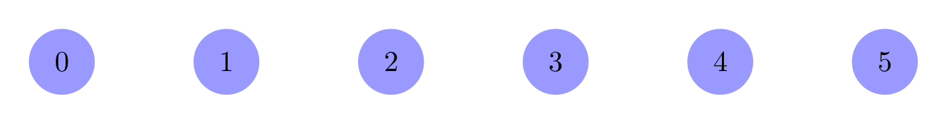
Show Tikz code
print(fig)% --------------------------------------------- %% Tikzfigure generated by tikzfigure v0.3.1 %% https://github.com/max-models/tikzfigure %% --------------------------------------------- %\begin{tikzpicture} % Row of circles \foreach \i in {0,1,...,5}{ \node[shape=circle, fill=blue!40, minimum size=0.8cm] (node0) at ({2 * \i}, {0}) {\i}; }\end{tikzpicture}print(fig.generate_standalone())\documentclass[border=10pt]{standalone}\PassOptionsToPackage{dvipsnames,svgnames,x11names}{xcolor}\usepackage{tikz}\usepackage{pgfplots}\pgfplotsset{compat=newest}\usepgfplotslibrary{groupplots}\usetikzlibrary{arrows.meta}\begin{document}% --------------------------------------------- %% Tikzfigure generated by tikzfigure v0.3.1 %% https://github.com/max-models/tikzfigure %% --------------------------------------------- %\begin{tikzpicture} % Row of circles \foreach \i in {0,1,...,5}{ \node[shape=circle, fill=blue!40, minimum size=0.8cm] (node0) at ({2 * \i}, {0}) {\i}; }\end{tikzpicture}
\end{document}Loop variable in colour expressions
Section titled “Loop variable in colour expressions”TikZ colour mixing expressions like blue!\i0!red interpolate between
two colours. Here \i ranges from 1 to 9, so \i0 gives 10, 20, … 90 —
a smooth gradient from blue to red.
fig = TikzFigure()
with fig.loop(    "i",    range(1, 10),    comment="Colour gradient",) as i:    fig.node(        (2 * i, 0),        shape="circle",        fill=r"blue!\i0!red",        content=i,        minimum_size="1cm",        color="white",        font=r"\bfseries",    )
fig.show()
Show Tikz code
print(fig)% --------------------------------------------- %% Tikzfigure generated by tikzfigure v0.3.1 %% https://github.com/max-models/tikzfigure %% --------------------------------------------- %\begin{tikzpicture} % Colour gradient \foreach \i in {1,2,...,9}{ \node[shape=circle, color=white, fill=blue!\i0!red, minimum size=1cm, font=\bfseries] (node0) at ({2 * \i}, {0}) {\i}; }\end{tikzpicture}print(fig.generate_standalone())\documentclass[border=10pt]{standalone}\PassOptionsToPackage{dvipsnames,svgnames,x11names}{xcolor}\usepackage{tikz}\usepackage{pgfplots}\pgfplotsset{compat=newest}\usepgfplotslibrary{groupplots}\usetikzlibrary{arrows.meta}\begin{document}% --------------------------------------------- %% Tikzfigure generated by tikzfigure v0.3.1 %% https://github.com/max-models/tikzfigure %% --------------------------------------------- %\begin{tikzpicture} % Colour gradient \foreach \i in {1,2,...,9}{ \node[shape=circle, color=white, fill=blue!\i0!red, minimum size=1cm, font=\bfseries] (node0) at ({2 * \i}, {0}) {\i}; }\end{tikzpicture}
\end{document}Nested loops: a 5x4 grid of nodes
Section titled “Nested loops: a 5x4 grid of nodes”Use a second fig.loop() inside the first to create a 2-D grid. The
inner loop variable \j is independent of the outer \i.
fig = TikzFigure()
with fig.loop(    "i",    range(5),    comment="Outer loop (columns)",) as i:    with fig.loop(        "j",        range(4),        comment="Inner loop (rows)",    ) as j:        fig.node(            (2 * i, 2 * j),            shape="rectangle",            fill="orange!30",            content=f"({i},{j})",            minimum_size="0.9cm",        )
fig.show()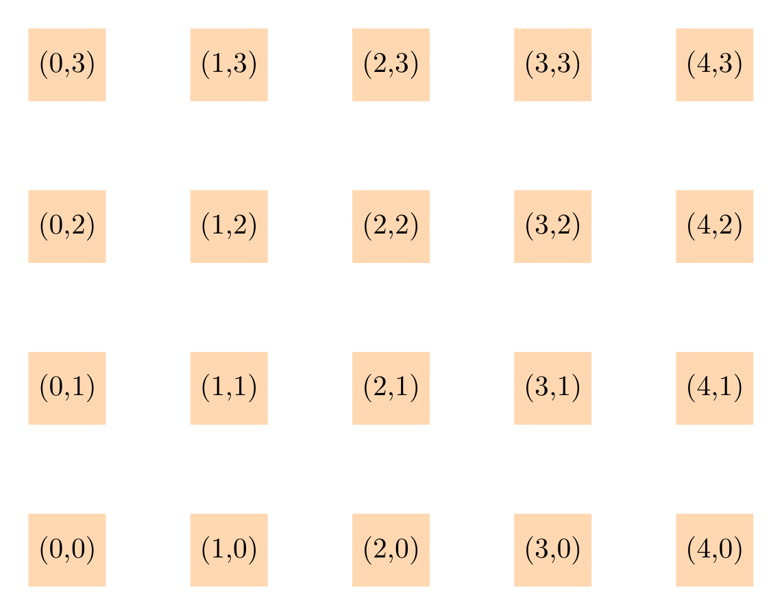
Show Tikz code
print(fig)% --------------------------------------------- %% Tikzfigure generated by tikzfigure v0.3.1 %% https://github.com/max-models/tikzfigure %% --------------------------------------------- %\begin{tikzpicture} % Outer loop (columns) \foreach \i in {0,1,...,4}{ % Inner loop (rows) \foreach \j in {0,1,...,3}{ \node[shape=rectangle, fill=orange!30, minimum size=0.9cm] (node0) at ({2 * \i}, {2 * \j}) {(\i,\j)}; } }\end{tikzpicture}print(fig.generate_standalone())\documentclass[border=10pt]{standalone}\PassOptionsToPackage{dvipsnames,svgnames,x11names}{xcolor}\usepackage{tikz}\usepackage{pgfplots}\pgfplotsset{compat=newest}\usepgfplotslibrary{groupplots}\usetikzlibrary{arrows.meta}\begin{document}% --------------------------------------------- %% Tikzfigure generated by tikzfigure v0.3.1 %% https://github.com/max-models/tikzfigure %% --------------------------------------------- %\begin{tikzpicture} % Outer loop (columns) \foreach \i in {0,1,...,4}{ % Inner loop (rows) \foreach \j in {0,1,...,3}{ \node[shape=rectangle, fill=orange!30, minimum size=0.9cm] (node0) at ({2 * \i}, {2 * \j}) {(\i,\j)}; } }\end{tikzpicture}
\end{document}The generated TikZ is a compact nested \foreach — compare that with
what 20 separate \node commands would look like.
variable: reusable TikZ constants
Section titled “variable: reusable TikZ constants”fig.variable(name, value) emits a \pgfmathsetmacro declaration at
the top of the picture. Use it to store a radius, spacing, or any
numeric constant that you want to be able to change in one place.
Here 12 nodes are placed on a circle of radius \radius. Python
computes the trigonometric coefficients; TikZ multiplies them by
\radius at compile time.
import math
fig = TikzFigure()fig.variable("radius", 3)
N = 12for i in range(N):    frac = round(i / N, 4)    angle = frac * 2 * math.pi    fig.node(        (f"{{\\radius*{math.cos(angle):.4f}}}", f"{{\\radius*{math.sin(angle):.4f}}}"),        shape="circle",        fill="teal!50",        content=str(i + 1),        minimum_size="0.7cm",        color="white",        font=r"\small",    )
fig.show()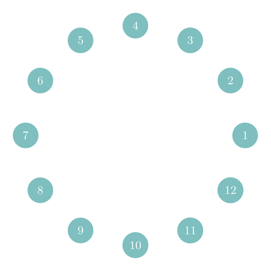
Show Tikz code
print(fig)% --------------------------------------------- %% Tikzfigure generated by tikzfigure v0.3.1 %% https://github.com/max-models/tikzfigure %% --------------------------------------------- %\begin{tikzpicture} \pgfmathsetmacro{\radius}{3} \node[shape=circle, color=white, fill=teal!50, minimum size=0.7cm, font=\small] (node0) at ({{\radius*1.0000}}, {{\radius*0.0000}}) {1}; \node[shape=circle, color=white, fill=teal!50, minimum size=0.7cm, font=\small] (node1) at ({{\radius*0.8661}}, {{\radius*0.4998}}) {2}; \node[shape=circle, color=white, fill=teal!50, minimum size=0.7cm, font=\small] (node2) at ({{\radius*0.4998}}, {{\radius*0.8661}}) {3}; \node[shape=circle, color=white, fill=teal!50, minimum size=0.7cm, font=\small] (node3) at ({{\radius*0.0000}}, {{\radius*1.0000}}) {4}; \node[shape=circle, color=white, fill=teal!50, minimum size=0.7cm, font=\small] (node4) at ({{\radius*-0.4998}}, {{\radius*0.8661}}) {5}; \node[shape=circle, color=white, fill=teal!50, minimum size=0.7cm, font=\small] (node5) at ({{\radius*-0.8661}}, {{\radius*0.4998}}) {6}; \node[shape=circle, color=white, fill=teal!50, minimum size=0.7cm, font=\small] (node6) at ({{\radius*-1.0000}}, {{\radius*0.0000}}) {7}; \node[shape=circle, color=white, fill=teal!50, minimum size=0.7cm, font=\small] (node7) at ({{\radius*-0.8661}}, {{\radius*-0.4998}}) {8}; \node[shape=circle, color=white, fill=teal!50, minimum size=0.7cm, font=\small] (node8) at ({{\radius*-0.4998}}, {{\radius*-0.8661}}) {9}; \node[shape=circle, color=white, fill=teal!50, minimum size=0.7cm, font=\small] (node9) at ({{\radius*-0.0000}}, {{\radius*-1.0000}}) {10}; \node[shape=circle, color=white, fill=teal!50, minimum size=0.7cm, font=\small] (node10) at ({{\radius*0.4998}}, {{\radius*-0.8661}}) {11}; \node[shape=circle, color=white, fill=teal!50, minimum size=0.7cm, font=\small] (node11) at ({{\radius*0.8661}}, {{\radius*-0.4998}}) {12};\end{tikzpicture}print(fig.generate_standalone())\documentclass[border=10pt]{standalone}\PassOptionsToPackage{dvipsnames,svgnames,x11names}{xcolor}\usepackage{tikz}\usepackage{pgfplots}\pgfplotsset{compat=newest}\usepgfplotslibrary{groupplots}\usetikzlibrary{arrows.meta}\begin{document}% --------------------------------------------- %% Tikzfigure generated by tikzfigure v0.3.1 %% https://github.com/max-models/tikzfigure %% --------------------------------------------- %\begin{tikzpicture} \pgfmathsetmacro{\radius}{3} \node[shape=circle, color=white, fill=teal!50, minimum size=0.7cm, font=\small] (node0) at ({{\radius*1.0000}}, {{\radius*0.0000}}) {1}; \node[shape=circle, color=white, fill=teal!50, minimum size=0.7cm, font=\small] (node1) at ({{\radius*0.8661}}, {{\radius*0.4998}}) {2}; \node[shape=circle, color=white, fill=teal!50, minimum size=0.7cm, font=\small] (node2) at ({{\radius*0.4998}}, {{\radius*0.8661}}) {3}; \node[shape=circle, color=white, fill=teal!50, minimum size=0.7cm, font=\small] (node3) at ({{\radius*0.0000}}, {{\radius*1.0000}}) {4}; \node[shape=circle, color=white, fill=teal!50, minimum size=0.7cm, font=\small] (node4) at ({{\radius*-0.4998}}, {{\radius*0.8661}}) {5}; \node[shape=circle, color=white, fill=teal!50, minimum size=0.7cm, font=\small] (node5) at ({{\radius*-0.8661}}, {{\radius*0.4998}}) {6}; \node[shape=circle, color=white, fill=teal!50, minimum size=0.7cm, font=\small] (node6) at ({{\radius*-1.0000}}, {{\radius*0.0000}}) {7}; \node[shape=circle, color=white, fill=teal!50, minimum size=0.7cm, font=\small] (node7) at ({{\radius*-0.8661}}, {{\radius*-0.4998}}) {8}; \node[shape=circle, color=white, fill=teal!50, minimum size=0.7cm, font=\small] (node8) at ({{\radius*-0.4998}}, {{\radius*-0.8661}}) {9}; \node[shape=circle, color=white, fill=teal!50, minimum size=0.7cm, font=\small] (node9) at ({{\radius*-0.0000}}, {{\radius*-1.0000}}) {10}; \node[shape=circle, color=white, fill=teal!50, minimum size=0.7cm, font=\small] (node10) at ({{\radius*0.4998}}, {{\radius*-0.8661}}) {11}; \node[shape=circle, color=white, fill=teal!50, minimum size=0.7cm, font=\small] (node11) at ({{\radius*0.8661}}, {{\radius*-0.4998}}) {12};\end{tikzpicture}
\end{document}Changing fig.variable("radius", 5) would scale the entire circle
without touching any node code.
Heart shape
Section titled “Heart shape”Remember the heart shape from the styling
tutorial? It can be drawn with a
single \draw command
width, height = 1.75, 2.0
fig = TikzFigure()
fig.colorlet("lightred", "red!40!white")fig.variable("width", 1.75)fig.variable("height", 2.0)
A = fig.node(r"-\width", r"\height")B = fig.node((0, 0))C = fig.node(r"\width", r"\height")D = fig.node(0, r"\height")
fig.draw(    A.to(B, options=["out=-90, in=135"])    .to(C, options=["out=45, in=-90"])    .to(D, options=["in=80, out=100"])    .to(A, options=["in=80, out=100"]),    color="red",    line_width=4,    cycle=True,    center=True,    fill="lightred",)
fig.show()
Practical example: a chain of labelled boxes
Section titled “Practical example: a chain of labelled boxes”A common diagram pattern is a horizontal chain of labelled boxes
connected by arrows. Using a \foreach loop keeps the LaTeX concise
even for long chains.
steps = ["Load", "Clean", "Transform", "Model", "Evaluate"]
fig = TikzFigure()
# Draw boxes via a TikZ foreach over a comma-separated list of indiceswith fig.loop(    "i",    range(len(steps)),    comment="Pipeline steps",) as loop:    loop.node(        (r"3*\i", 0),        shape="rectangle",        fill="blue!20",        draw="blue!60",        minimum_width="2.2cm",        minimum_height="0.8cm",        rounded_corners="4pt",        line_width=1.5,    )
# Add step labels in Python (strings can't live inside \foreach easily)for i, step in enumerate(steps):    fig.node(        (i * 3, 0),        content=step,        draw="none",        font=r"\small\bfseries",    )
# Draw arrows between boxesfor i in range(len(steps) - 1):    fig.draw(        [(i * 3 + 1.1, 0), (i * 3 + 1.9, 0)],        arrows=arrows.forward,        line_width=1.5,        color="blue!60",    )
fig.show()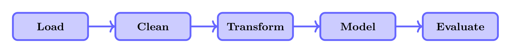
Show Tikz code
print(fig)% --------------------------------------------- %% Tikzfigure generated by tikzfigure v0.3.1 %% https://github.com/max-models/tikzfigure %% --------------------------------------------- %\begin{tikzpicture} % Pipeline steps \foreach \i in {0,1,...,4}{ \node[shape=rectangle, fill=blue!20, draw=blue!60, minimum width=2.2cm, minimum height=0.8cm, line width=1.5, rounded corners=4pt] () at ({3*\i}, {0}) {}; } \node[draw=none, font=\small\bfseries] (node0) at ({0}, {0}) {Load}; \node[draw=none, font=\small\bfseries] (node1) at ({3}, {0}) {Clean}; \node[draw=none, font=\small\bfseries] (node2) at ({6}, {0}) {Transform}; \node[draw=none, font=\small\bfseries] (node3) at ({9}, {0}) {Model}; \node[draw=none, font=\small\bfseries] (node4) at ({12}, {0}) {Evaluate}; \draw[->, color=blue!60, line width=1.5] (1.1, 0) to (1.9, 0); \draw[->, color=blue!60, line width=1.5] (4.1, 0) to (4.9, 0); \draw[->, color=blue!60, line width=1.5] (7.1, 0) to (7.9, 0); \draw[->, color=blue!60, line width=1.5] (10.1, 0) to (10.9, 0);\end{tikzpicture}print(fig.generate_standalone())\documentclass[border=10pt]{standalone}\PassOptionsToPackage{dvipsnames,svgnames,x11names}{xcolor}\usepackage{tikz}\usepackage{pgfplots}\pgfplotsset{compat=newest}\usepgfplotslibrary{groupplots}\usetikzlibrary{arrows.meta}\begin{document}% --------------------------------------------- %% Tikzfigure generated by tikzfigure v0.3.1 %% https://github.com/max-models/tikzfigure %% --------------------------------------------- %\begin{tikzpicture} % Pipeline steps \foreach \i in {0,1,...,4}{ \node[shape=rectangle, fill=blue!20, draw=blue!60, minimum width=2.2cm, minimum height=0.8cm, line width=1.5, rounded corners=4pt] () at ({3*\i}, {0}) {}; } \node[draw=none, font=\small\bfseries] (node0) at ({0}, {0}) {Load}; \node[draw=none, font=\small\bfseries] (node1) at ({3}, {0}) {Clean}; \node[draw=none, font=\small\bfseries] (node2) at ({6}, {0}) {Transform}; \node[draw=none, font=\small\bfseries] (node3) at ({9}, {0}) {Model}; \node[draw=none, font=\small\bfseries] (node4) at ({12}, {0}) {Evaluate}; \draw[->, color=blue!60, line width=1.5] (1.1, 0) to (1.9, 0); \draw[->, color=blue!60, line width=1.5] (4.1, 0) to (4.9, 0); \draw[->, color=blue!60, line width=1.5] (7.1, 0) to (7.9, 0); \draw[->, color=blue!60, line width=1.5] (10.1, 0) to (10.9, 0);\end{tikzpicture}
\end{document}