3D Figures

tikzfigure supports 3-D plots via fig.plot3d(xvec, yvec, zvec). Pass ndim=3 when creating the figure to switch to pgfplots’ \begin{axis} environment with a default perspective of view={20}{30}.

Key facts: - Multiple plot3d calls on the same figure stack as separate curves. - add_node(x, y, z=z, ...) places a marker in 3-D space. - show_axes=True adds labelled axis lines and a grid.

This tutorial covers: - Simple helix - the minimal 3-D setup - Torus knot - a parametric knot wound on a torus surface - Double helix - two interleaved helices with connecting rungs - Sphere wireframe - a sphere assembled from many short plot3d curves - Butterfly effect - two nearby Lorenz trajectories diverging over time

import numpy as np
from scipy.integrate import odeint

from tikzfigure import TikzFigure

A simple 3-D helix

Before tackling the Lorenz system, here is a simple parametric helix to illustrate the 3-D setup.

fig = TikzFigure(ndim=3)

t = np.linspace(0, 4 * np.pi, 200)
xvec = np.cos(t)
yvec = np.sin(t)
zvec = t / (4 * np.pi) * 4  # rise from 0 to 4

fig.plot3d(xvec, yvec, zvec, options=["color=blue", "thick"], layer=0)

# Mark start and end
fig.add_node(
    x=xvec[0],
    y=yvec[0],
    z=zvec[0],
    fill="green!60!black",
    inner_sep="3pt",
    options="circle",
)
fig.add_node(
    x=xvec[-1],
    y=yvec[-1],
    z=zvec[-1],
    fill="red!70!black",
    inner_sep="3pt",
    options="circle",
)

fig.show(width=400)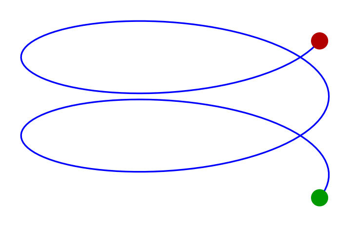

Lorenz attractor

The Lorenz system is the ODE, based on this example:

$\dot x = \sigma(y - x), \quad \dot y = x(\rho - z) - y, \quad \dot z = xy - \beta z$

with $\sigma = 10$, $\rho = 28$, $\beta = 8/3$. Small differences in initial conditions lead to wildly different trajectories - the butterfly effect.

We integrate for 20 time units, scale the result down, and plot the trajectory. The green dot marks the start; red marks the end.

rho, sigma, beta = 28.0, 10.0, 8.0 / 3.0


def lorenz(state, t):
    x, y, z = state
    return [sigma * (y - x), x * (rho - z) - y, x * y - beta * z]


t = np.arange(0.0, 20.0, 0.01)
states = odeint(lorenz, y0=[1.0, 1.0, 1.0], t=t) * 0.25

fig = TikzFigure(ndim=3)

fig.plot3d(states[:, 0], states[:, 1], states[:, 2], color="black", thick=True, layer=0)

fig.add_node(
    x=states[0, 0],
    y=states[0, 1],
    z=states[0, 2],
    fill="green!50!black",
    inner_sep="2.0pt",
    options="circle",
)
fig.add_node(
    x=states[-1, 0],
    y=states[-1, 1],
    z=states[-1, 2],
    fill="red!50!black",
    inner_sep="2.0pt",
    options="circle",
)

fig.show(width=500)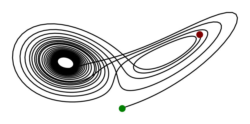

Torus knot

A $(p, q)$ torus knot winds $p$ times around the torus in the longitudinal direction and $q$ times in the meridional direction. The parametric equations are:

y(t) = (R + r\cos(qt))\sin(pt), \quad z(t) = r\sin(qt)$$ With $p=2, q=3$ we get the **trefoil knot** - the simplest non-trivial knot. Increasing $p$ and $q$ produces more complex knots; try $(3, 5)$ or $(4, 7)$. ``` python fig = TikzFigure(ndim=3) p, q = 2, 3 # (2,3) = trefoil knot R, r = 2.0, 0.8 # torus major / minor radii t = np.linspace(0, 2 * np.pi, 600) x = (R + r * np.cos(q * t)) * np.cos(p * t) y = (R + r * np.cos(q * t)) * np.sin(p * t) z = r * np.sin(q * t) fig.plot3d(x, y, z, options=["color=purple", "thick"], layer=0) fig.show(width=450) ``` <img src="/tikzfigure/tutorials/tutorial_08_3d_figures/figure-commonmark/cell-5-output-1.png" width="450" />