Spy library
This tutorial introduces the dedicated spy API for inset zoom views and magnified regions.
The examples now start simple and then build up:
- one basic spy inset on a small drawing
- custom spy-in node shapes and sizes
- figure-wide defaults with
configure_spy_scope(...) - the classic pgfplots spy example from the TikZ manual
- local spy defaults with
spy_scope(...) - nested spy scopes with a custom connection path
from tikzfigure import TikzFigure, colors, shapesA minimal spy example
Section titled “A minimal spy example”The smallest useful pattern is just a drawing plus one spy inset. fig.spy(...)
automatically enables a basic spy scope on the figure.
fig = TikzFigure()
fig.draw([(-0.3, 0), (2.8, 0)], color=colors.black, line_width="0.8pt")fig.draw([(0, -0.8), (0, 1.2)], color=colors.lightgray)fig.draw([(1.2, -0.6), (1.2, 0.9)], color=colors.lightgray)fig.draw([(0, 0), (2.2, 0.8)], color=colors.blue, line_width="1.1pt")
fig.spy(    on=(1.2, 0.45),    at=(4.0, 0.9),    magnification=3,    size="1.3cm",)
fig.show()
/home/runner/work/tikzfigure/tikzfigure/.venv/lib/python3.12/site-packages/fitz/__init__.py:17: FutureWarning: The `fitz` API is deprecated and will be removed in future. Use `import pymupdf` instead. warnings.warn(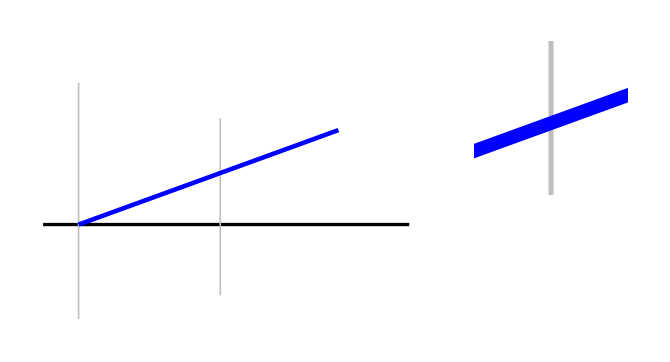
Show the TikZ code
% --------------------------------------------- %% Tikzfigure generated by tikzfigure v0.5.0 %% https://github.com/max-models/tikzfigure %% --------------------------------------------- %\begin{tikzpicture}[spy scope] \draw[color=black, line width=0.8pt] (-0.3, 0) to (2.8, 0); \draw[color=lightgray] (0, -0.8) to (0, 1.2); \draw[color=lightgray] (1.2, -0.6) to (1.2, 0.9); \draw[color=blue, line width=1.1pt] (0, 0) to (2.2, 0.8); \spy[magnification=3, size=1.3cm] on ({1.2}, {0.45}) in node at ({4.0}, {0.9});\end{tikzpicture}Show the standalone LaTeX document
\documentclass[border=10pt]{standalone}\PassOptionsToPackage{dvipsnames,svgnames,x11names}{xcolor}\usepackage{tikz}\usepackage{pgfplots}\pgfplotsset{compat=newest}\usepgfplotslibrary{groupplots}\usetikzlibrary{arrows.meta,spy}\begin{document}% --------------------------------------------- %% Tikzfigure generated by tikzfigure v0.5.0     %% https://github.com/max-models/tikzfigure      %% --------------------------------------------- %\begin{tikzpicture}[spy scope]    \draw[color=black, line width=0.8pt] (-0.3, 0) to (2.8, 0);    \draw[color=lightgray] (0, -0.8) to (0, 1.2);    \draw[color=lightgray] (1.2, -0.6) to (1.2, 0.9);    \draw[color=blue, line width=1.1pt] (0, 0) to (2.2, 0.8);    \spy[magnification=3, size=1.3cm] on ({1.2}, {0.45}) in node at ({4.0}, {0.9});\end{tikzpicture}
\end{document}
This already gives you the core spy behavior:
on=...picks the center of the region to magnifyat=...places the inset nodemagnification=controls zoomsize=controls the inset size
Customizing the spy-in node
Section titled “Customizing the spy-in node”You can style the spy-in node just like a normal TikZ node. Here we use a small zig-zag path and highlight two different details.
fig = TikzFigure()
ridge = [(-0.2, 0), (0.8, 0.9), (1.5, 0.3), (2.3, 1.1), (3.0, 0.5)]fig.draw(ridge, color=colors.black, line_width="1pt")
for point in ridge:    fig.node(        point,        shape="circle",        minimum_size="4pt",        inner_sep="0pt",        fill=colors.orange.mix(percent=20),        draw=colors.black,    )
fig.spy(    on=(0.8, 0.9),    at=(4.4, 1.1),    options=[colors.red],    magnification=4,    size="1.35cm",    connect_spies=True,    node_options=[shapes.circle],    node_style={"draw": colors.red, "line_width": "0.8pt", "fill": colors.white},)
fig.spy(    on=(2.3, 1.1),    at=(4.3, -0.2),    options=[colors.blue],    magnification=5,    width="1.8cm",    height="1.0cm",    node_label="peak detail",    node_options=[shapes.rectangle],    node_style={        "draw": colors.blue,        "rounded_corners": "2pt",        "fill": colors.white,    },)
fig.show()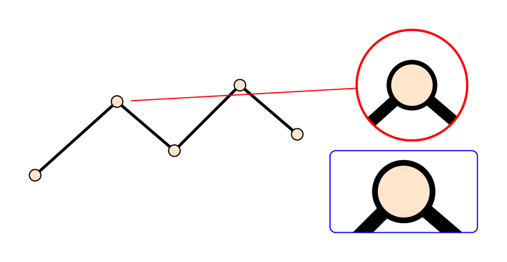
Show the TikZ code
% --------------------------------------------- %% Tikzfigure generated by tikzfigure v0.5.0 %% https://github.com/max-models/tikzfigure %% --------------------------------------------- %\begin{tikzpicture}[spy scope] \draw[color=black, line width=1pt] (-0.2, 0) to (0.8, 0.9) to (1.5, 0.3) to (2.3, 1.1) to (3.0, 0.5); \node[shape=circle, fill=orange!20!white, draw=black, minimum size=4pt, inner sep=0pt] (node0) at ({-0.2}, {0}) {}; \node[shape=circle, fill=orange!20!white, draw=black, minimum size=4pt, inner sep=0pt] (node1) at ({0.8}, {0.9}) {}; \node[shape=circle, fill=orange!20!white, draw=black, minimum size=4pt, inner sep=0pt] (node2) at ({1.5}, {0.3}) {}; \node[shape=circle, fill=orange!20!white, draw=black, minimum size=4pt, inner sep=0pt] (node3) at ({2.3}, {1.1}) {}; \node[shape=circle, fill=orange!20!white, draw=black, minimum size=4pt, inner sep=0pt] (node4) at ({3.0}, {0.5}) {}; \spy[red, connect spies, magnification=4, size=1.35cm] on ({0.8}, {0.9}) in node [circle, draw=red, line width=0.8pt, fill=white] at ({4.4}, {1.1}); \spy[blue, magnification=5, width=1.8cm, height=1.0cm] on ({2.3}, {1.1}) in node (peak detail) [rectangle, draw=blue, rounded corners=2pt, fill=white] at ({4.3}, {-0.2});\end{tikzpicture}Show the standalone LaTeX document
\documentclass[border=10pt]{standalone}\PassOptionsToPackage{dvipsnames,svgnames,x11names}{xcolor}\usepackage{tikz}\usepackage{pgfplots}\pgfplotsset{compat=newest}\usepgfplotslibrary{groupplots}\usetikzlibrary{arrows.meta,spy}\begin{document}% --------------------------------------------- %% Tikzfigure generated by tikzfigure v0.5.0     %% https://github.com/max-models/tikzfigure      %% --------------------------------------------- %\begin{tikzpicture}[spy scope]    \draw[color=black, line width=1pt] (-0.2, 0)        to        (0.8, 0.9)        to        (1.5, 0.3)        to        (2.3, 1.1)        to        (3.0, 0.5);    \node[shape=circle, fill=orange!20!white, draw=black, minimum size=4pt, inner sep=0pt] (node0) at ({-0.2}, {0}) {};    \node[shape=circle, fill=orange!20!white, draw=black, minimum size=4pt, inner sep=0pt] (node1) at ({0.8}, {0.9}) {};    \node[shape=circle, fill=orange!20!white, draw=black, minimum size=4pt, inner sep=0pt] (node2) at ({1.5}, {0.3}) {};    \node[shape=circle, fill=orange!20!white, draw=black, minimum size=4pt, inner sep=0pt] (node3) at ({2.3}, {1.1}) {};    \node[shape=circle, fill=orange!20!white, draw=black, minimum size=4pt, inner sep=0pt] (node4) at ({3.0}, {0.5}) {};    \spy[red, connect spies, magnification=4, size=1.35cm] on ({0.8}, {0.9}) in node [circle, draw=red, line width=0.8pt, fill=white] at ({4.4}, {1.1});    \spy[blue, magnification=5, width=1.8cm, height=1.0cm] on ({2.3}, {1.1}) in node (peak detail) [rectangle, draw=blue, rounded corners=2pt, fill=white] at ({4.3}, {-0.2});\end{tikzpicture}
\end{document}
This adds a few new pieces:
connect_spies=Truedraws the default connectornode_options=[...]controls flag-style node options like shapesnode_style={...}controls keyword-style node options likedraw=...node_label="peak detail"names the spy-in nodewidth=andheight=let you use non-square spy nodes
Figure-wide defaults with configure_spy_scope(...)
Section titled “Figure-wide defaults with configure_spy_scope(...)”If several spies in the same figure should share defaults, configure the
tikzpicture-level spy scope once and then use fig.spy(...) repeatedly.
This simple city-block map uses the same inset style for multiple locations.
fig = TikzFigure()
fig.configure_spy_scope(    mode="outlines",    options=[shapes.rectangle],    magnification=4,    width="1.9cm",    height="1.0cm",    connect_spies=True,    every_spy_in_node_style={        "draw": colors.green.mix(colors.black, percent=35),        "fill": colors.white,        "rounded_corners": "2pt",    },    every_spy_on_node_style={        "draw": colors.green.mix(colors.black, percent=15),        "fill": colors.green,        "fill_opacity": 0.08,    },)
fig.draw(    [(-0.2, -0.2), (4.8, -0.2), (4.8, 3.2), (-0.2, 3.2)],    cycle=True,    fill=colors.gray.mix(percent=12),    draw="none",)
for x in [1.4, 3.2]:    fig.draw([(x, -0.2), (x, 3.2)], color=colors.white, line_width="10pt")for y in [1.0, 2.2]:    fig.draw([(-0.2, y), (4.8, y)], color=colors.white, line_width="10pt")
blocks = [    ((0.15, 0.15), (1.05, 0.75), colors.orange.mix(percent=18), "cafe"),    ((1.75, 0.15), (2.85, 0.75), colors.blue.mix(percent=14), "library"),    ((3.55, 0.15), (4.45, 0.75), colors.red.mix(percent=12), "gallery"),    ((0.15, 1.35), (1.05, 2.95), colors.green.mix(percent=16), "park"),    ((1.75, 1.35), (2.85, 2.95), colors.yellow.mix(percent=16), "market"),    ((3.55, 1.35), (4.45, 2.95), colors.purple.mix(percent=10), "museum"),]
for lower_left, upper_right, fill_color, label in blocks:    x0, y0 = lower_left    x1, y1 = upper_right    fig.draw(        [(x0, y0), (x1, y0), (x1, y1), (x0, y1)],        cycle=True,        rounded_corners="2pt",        fill=fill_color,        draw=fill_color.mix(colors.black, percent=20),    )    fig.node(((x0 + x1) / 2, (y0 + y1) / 2), content=label, draw="none", font=r"\small")
fig.spy(on=(0.55, 2.1), at=(6.4, 2.45), options=[colors.green])fig.spy(on=(2.3, 2.15), at=(6.4, 0.8), options=[colors.orange])
fig.show()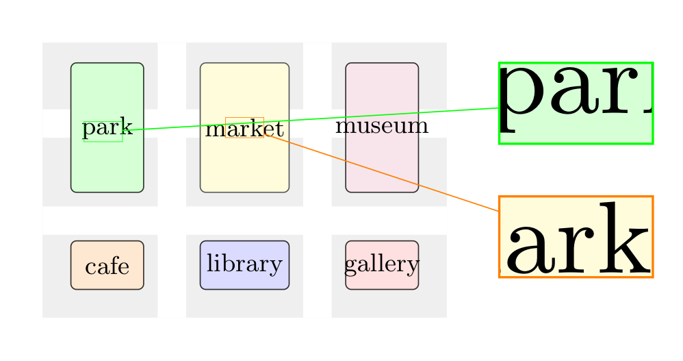
Show the TikZ code
% --------------------------------------------- %% Tikzfigure generated by tikzfigure v0.5.0 %% https://github.com/max-models/tikzfigure %% --------------------------------------------- %\begin{tikzpicture}[spy using outlines={rectangle, connect spies, magnification=4, width=1.9cm, height=1.0cm}, every spy in node/.style={draw=green!35!black, fill=white, rounded corners=2pt}, every spy on node/.style={draw=green!15!black, fill=green, fill opacity=0.08}] \draw[fill=gray!12!white, draw=none] (-0.2, -0.2) to (4.8, -0.2) to (4.8, 3.2) to (-0.2, 3.2) -- cycle; \draw[color=white, line width=10pt] (1.4, -0.2) to (1.4, 3.2); \draw[color=white, line width=10pt] (3.2, -0.2) to (3.2, 3.2); \draw[color=white, line width=10pt] (-0.2, 1.0) to (4.8, 1.0); \draw[color=white, line width=10pt] (-0.2, 2.2) to (4.8, 2.2); \draw[fill=orange!18!white, draw=orange!18!white!20!black, rounded corners=2pt] (0.15, 0.15) to (1.05, 0.15) to (1.05, 0.75) to (0.15, 0.75) -- cycle; \node[draw=none, font=\small] (node0) at ({0.6}, {0.45}) {cafe}; \draw[fill=blue!14!white, draw=blue!14!white!20!black, rounded corners=2pt] (1.75, 0.15) to (2.85, 0.15) to (2.85, 0.75) to (1.75, 0.75) -- cycle; \node[draw=none, font=\small] (node1) at ({2.3}, {0.45}) {library}; \draw[fill=red!12!white, draw=red!12!white!20!black, rounded corners=2pt] (3.55, 0.15) to (4.45, 0.15) to (4.45, 0.75) to (3.55, 0.75) -- cycle; \node[draw=none, font=\small] (node2) at ({4.0}, {0.45}) {gallery}; \draw[fill=green!16!white, draw=green!16!white!20!black, rounded corners=2pt] (0.15, 1.35) to (1.05, 1.35) to (1.05, 2.95) to (0.15, 2.95) -- cycle; \node[draw=none, font=\small] (node3) at ({0.6}, {2.1500000000000004}) {park}; \draw[fill=yellow!16!white, draw=yellow!16!white!20!black, rounded corners=2pt] (1.75, 1.35) to (2.85, 1.35) to (2.85, 2.95) to (1.75, 2.95) -- cycle; \node[draw=none, font=\small] (node4) at ({2.3}, {2.1500000000000004}) {market}; \draw[fill=purple!10!white, draw=purple!10!white!20!black, rounded corners=2pt] (3.55, 1.35) to (4.45, 1.35) to (4.45, 2.95) to (3.55, 2.95) -- cycle; \node[draw=none, font=\small] (node5) at ({4.0}, {2.1500000000000004}) {museum}; \spy[green] on ({0.55}, {2.1}) in node at ({6.4}, {2.45}); \spy[orange] on ({2.3}, {2.15}) in node at ({6.4}, {0.8});\end{tikzpicture}Show the standalone LaTeX document
\documentclass[border=10pt]{standalone}\PassOptionsToPackage{dvipsnames,svgnames,x11names}{xcolor}\usepackage{tikz}\usepackage{pgfplots}\pgfplotsset{compat=newest}\usepgfplotslibrary{groupplots}\usetikzlibrary{arrows.meta,spy}\begin{document}% --------------------------------------------- %% Tikzfigure generated by tikzfigure v0.5.0     %% https://github.com/max-models/tikzfigure      %% --------------------------------------------- %\begin{tikzpicture}[spy using outlines={rectangle, connect spies, magnification=4, width=1.9cm, height=1.0cm}, every spy in node/.style={draw=green!35!black, fill=white, rounded corners=2pt}, every spy on node/.style={draw=green!15!black, fill=green, fill opacity=0.08}]    \draw[fill=gray!12!white, draw=none] (-0.2, -0.2)        to        (4.8, -0.2)        to        (4.8, 3.2)        to        (-0.2, 3.2) -- cycle;    \draw[color=white, line width=10pt] (1.4, -0.2) to (1.4, 3.2);    \draw[color=white, line width=10pt] (3.2, -0.2) to (3.2, 3.2);    \draw[color=white, line width=10pt] (-0.2, 1.0) to (4.8, 1.0);    \draw[color=white, line width=10pt] (-0.2, 2.2) to (4.8, 2.2);    \draw[fill=orange!18!white, draw=orange!18!white!20!black, rounded corners=2pt] (0.15, 0.15)        to        (1.05, 0.15)        to        (1.05, 0.75)        to        (0.15, 0.75) -- cycle;    \node[draw=none, font=\small] (node0) at ({0.6}, {0.45}) {cafe};    \draw[fill=blue!14!white, draw=blue!14!white!20!black, rounded corners=2pt] (1.75, 0.15)        to        (2.85, 0.15)        to        (2.85, 0.75)        to        (1.75, 0.75) -- cycle;    \node[draw=none, font=\small] (node1) at ({2.3}, {0.45}) {library};    \draw[fill=red!12!white, draw=red!12!white!20!black, rounded corners=2pt] (3.55, 0.15)        to        (4.45, 0.15)        to        (4.45, 0.75)        to        (3.55, 0.75) -- cycle;    \node[draw=none, font=\small] (node2) at ({4.0}, {0.45}) {gallery};    \draw[fill=green!16!white, draw=green!16!white!20!black, rounded corners=2pt] (0.15, 1.35)        to        (1.05, 1.35)        to        (1.05, 2.95)        to        (0.15, 2.95) -- cycle;    \node[draw=none, font=\small] (node3) at ({0.6}, {2.1500000000000004}) {park};    \draw[fill=yellow!16!white, draw=yellow!16!white!20!black, rounded corners=2pt] (1.75, 1.35)        to        (2.85, 1.35)        to        (2.85, 2.95)        to        (1.75, 2.95) -- cycle;    \node[draw=none, font=\small] (node4) at ({2.3}, {2.1500000000000004}) {market};    \draw[fill=purple!10!white, draw=purple!10!white!20!black, rounded corners=2pt] (3.55, 1.35)        to        (4.45, 1.35)        to        (4.45, 2.95)        to        (3.55, 2.95) -- cycle;    \node[draw=none, font=\small] (node5) at ({4.0}, {2.1500000000000004}) {museum};    \spy[green] on ({0.55}, {2.1}) in node at ({6.4}, {2.45});    \spy[orange] on ({2.3}, {2.15}) in node at ({6.4}, {0.8});\end{tikzpicture}
\end{document}
This is a good pattern when you want:
- the same magnification for all spies
- the same inset shape and border styling
- the same spy-on styling
Reproducing the classic pgfplots spy example
Section titled “Reproducing the classic pgfplots spy example”Here is the classic pgfplots example from the TikZ manual, reproduced using only the Python API.
fig = TikzFigure()
fig.configure_spy_scope(    mode="outlines",    options=[shapes.rectangle],    magnification=3,    connect_spies=True,)
ax = fig.axis2d(    xlim=(-5, 5),    grid="major",    options=["no markers"],    domain="-5:5",    enlargelimits="false",)
ax.add_plot(func="x^2", color=colors.red)ax.add_plot(func="x^3", color=colors.blue)
spypoint = ax.coordinate("spypoint", at="axis cs:0,0")spyviewer = ax.coordinate("spyviewer", at="axis cs:0.5,-90")ax.spy(    on=spypoint,    at=spyviewer,    width="6cm",    height="1cm",    node_style={"fill": colors.white},)
fig.show()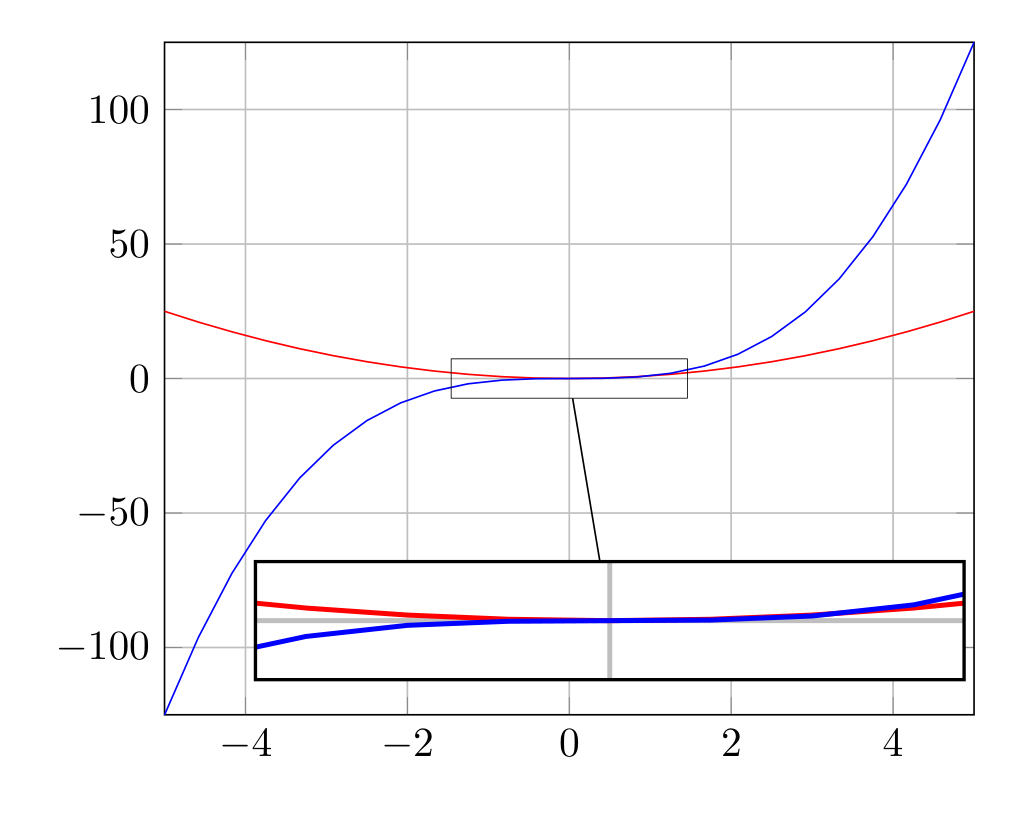
Show the TikZ code
% --------------------------------------------- %% Tikzfigure generated by tikzfigure v0.5.0 %% https://github.com/max-models/tikzfigure %% --------------------------------------------- %\begin{tikzpicture}[spy using outlines={rectangle, connect spies, magnification=3}] \begin{axis}[no markers, xmin=-5, xmax=5, grid=major, domain=-5:5, enlargelimits=false] \addplot[color=red] {x^2}; \addplot[color=blue] {x^3}; \coordinate (spypoint) at (axis cs:0,0); \coordinate (spyviewer) at (axis cs:0.5,-90); \spy[width=6cm, height=1cm] on (spypoint) in node [fill=white] at (spyviewer); \end{axis}\end{tikzpicture}Show the standalone LaTeX document
\documentclass[border=10pt]{standalone}\PassOptionsToPackage{dvipsnames,svgnames,x11names}{xcolor}\usepackage{tikz}\usepackage{pgfplots}\pgfplotsset{compat=newest}\usepgfplotslibrary{groupplots}\usetikzlibrary{arrows.meta,spy}\usepackage{pgfplots}\begin{document}% --------------------------------------------- %% Tikzfigure generated by tikzfigure v0.5.0     %% https://github.com/max-models/tikzfigure      %% --------------------------------------------- %\begin{tikzpicture}[spy using outlines={rectangle, connect spies, magnification=3}]    \begin{axis}[no markers, xmin=-5, xmax=5, grid=major, domain=-5:5, enlargelimits=false]        \addplot[color=red] {x^2};        \addplot[color=blue] {x^3};        \coordinate (spypoint) at (axis cs:0,0);        \coordinate (spyviewer) at (axis cs:0.5,-90);        \spy[width=6cm, height=1cm] on (spypoint) in node [fill=white] at (spyviewer);    \end{axis}\end{tikzpicture}
\end{document}
This matches the original idea closely:
mode="outlines"maps tospy using outlines={...}options=[shapes.rectangle]makes the inset rectangularax.coordinate(...)andax.spy(...)keep everything inside theaxisenvironment
Local spy defaults with spy_scope(...)
Section titled “Local spy defaults with spy_scope(...)”Use spy_scope(...) when spy settings should only apply to part of the figure.
This mirrors the TikZ manual more closely than a figure-wide spy scope.
Here the spy scope is used on a small transit-map sketch, and one spy zooms in
directly on a labeled Node object.
def add_station(scope, position, size="3pt", fill=colors.white, label=None):    return scope.node(        position,        label=label,        shape="circle",        minimum_size=size,        inner_sep="0pt",        fill=fill,        draw=colors.black,        line_width="0.3pt",    )

fig = TikzFigure()
with fig.spy_scope(    mode="outlines",    options=[shapes.circle],    magnification=4,    size="1.5cm",    connect_spies=True,    every_spy_in_node_options=[shapes.circle],    every_spy_in_node_style={        "draw": colors.orange.mix(colors.black, percent=28),        "line_width": "0.9pt",        "fill": colors.white,    },    every_spy_on_node_options=[shapes.circle],    every_spy_on_node_style={        "draw": colors.orange.mix(colors.black, percent=18),        "fill": colors.orange,        "fill_opacity": 0.08,    },) as metro:    red_line = [(-0.1, -0.5), (0.9, 0.1), (1.9, 0.7), (3.0, 1.2), (4.0, 1.55)]    blue_line = [(0.1, 1.35), (1.1, 0.95), (2.0, 0.65), (3.1, 0.1), (4.1, -0.4)]
    for line_points, line_color in [(red_line, colors.red), (blue_line, colors.blue)]:        metro.draw(line_points, color=line_color, line_width="2.6pt")        for point in line_points:            add_station(metro, point)
    central = add_station(        metro,        (2.0, 0.65),        size="5pt",        fill=colors.yellow.mix(percent=18),        label="central_hub",    )    metro.node((2.0, 0.2), content="Central", draw="none", font=r"\small\bfseries")
    metro.spy(        on=central,        at=(5.7, 1.2),        options=[colors.orange],        node_label="central interchange",    )    metro.spy(        on=(3.95, 1.5),        at=(5.7, -0.45),        options=[colors.blue],        width="1.8cm",        height="1.0cm",        node_options=[shapes.rectangle],        node_style={            "draw": colors.blue,            "rounded_corners": "2pt",            "fill": colors.white,        },    )
fig.show()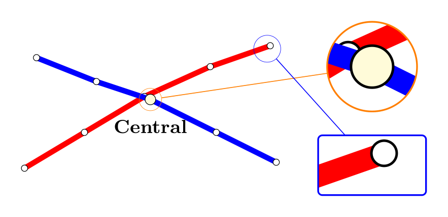
Show the TikZ code
% --------------------------------------------- %% Tikzfigure generated by tikzfigure v0.5.0 %% https://github.com/max-models/tikzfigure %% --------------------------------------------- %\begin{tikzpicture} \begin{scope}[spy using outlines={circle, connect spies, magnification=4, size=1.5cm}, every spy in node/.style={circle, draw=orange!28!black, line width=0.9pt, fill=white}, every spy on node/.style={circle, draw=orange!18!black, fill=orange, fill opacity=0.08}] \draw[color=red, line width=2.6pt] (-0.1, -0.5) to (0.9, 0.1) to (1.9, 0.7) to (3.0, 1.2) to (4.0, 1.55); \node[shape=circle, fill=white, draw=black, minimum size=3pt, inner sep=0pt, line width=0.3pt] (None) at ({-0.1}, {-0.5}) {}; \node[shape=circle, fill=white, draw=black, minimum size=3pt, inner sep=0pt, line width=0.3pt] (None) at ({0.9}, {0.1}) {}; \node[shape=circle, fill=white, draw=black, minimum size=3pt, inner sep=0pt, line width=0.3pt] (None) at ({1.9}, {0.7}) {}; \node[shape=circle, fill=white, draw=black, minimum size=3pt, inner sep=0pt, line width=0.3pt] (None) at ({3.0}, {1.2}) {}; \node[shape=circle, fill=white, draw=black, minimum size=3pt, inner sep=0pt, line width=0.3pt] (None) at ({4.0}, {1.55}) {}; \draw[color=blue, line width=2.6pt] (0.1, 1.35) to (1.1, 0.95) to (2.0, 0.65) to (3.1, 0.1) to (4.1, -0.4); \node[shape=circle, fill=white, draw=black, minimum size=3pt, inner sep=0pt, line width=0.3pt] (None) at ({0.1}, {1.35}) {}; \node[shape=circle, fill=white, draw=black, minimum size=3pt, inner sep=0pt, line width=0.3pt] (None) at ({1.1}, {0.95}) {}; \node[shape=circle, fill=white, draw=black, minimum size=3pt, inner sep=0pt, line width=0.3pt] (None) at ({2.0}, {0.65}) {}; \node[shape=circle, fill=white, draw=black, minimum size=3pt, inner sep=0pt, line width=0.3pt] (None) at ({3.1}, {0.1}) {}; \node[shape=circle, fill=white, draw=black, minimum size=3pt, inner sep=0pt, line width=0.3pt] (None) at ({4.1}, {-0.4}) {}; \node[shape=circle, fill=yellow!18!white, draw=black, minimum size=5pt, inner sep=0pt, line width=0.3pt] (central_hub) at ({2.0}, {0.65}) {}; \node[draw=none, font=\small\bfseries] () at ({2.0}, {0.2}) {Central}; \spy[orange] on (central_hub) in node (central interchange) at ({5.7}, {1.2}); \spy[blue, width=1.8cm, height=1.0cm] on ({3.95}, {1.5}) in node [rectangle, draw=blue, rounded corners=2pt, fill=white] at ({5.7}, {-0.45}); \end{scope}\end{tikzpicture}Show the standalone LaTeX document
\documentclass[border=10pt]{standalone}\PassOptionsToPackage{dvipsnames,svgnames,x11names}{xcolor}\usepackage{tikz}\usepackage{pgfplots}\pgfplotsset{compat=newest}\usepgfplotslibrary{groupplots}\usetikzlibrary{arrows.meta,spy}\begin{document}% --------------------------------------------- %% Tikzfigure generated by tikzfigure v0.5.0     %% https://github.com/max-models/tikzfigure      %% --------------------------------------------- %\begin{tikzpicture}    \begin{scope}[spy using outlines={circle, connect spies, magnification=4, size=1.5cm}, every spy in node/.style={circle, draw=orange!28!black, line width=0.9pt, fill=white}, every spy on node/.style={circle, draw=orange!18!black, fill=orange, fill opacity=0.08}]        \draw[color=red, line width=2.6pt] (-0.1, -0.5)            to            (0.9, 0.1)            to            (1.9, 0.7)            to            (3.0, 1.2)            to            (4.0, 1.55);        \node[shape=circle, fill=white, draw=black, minimum size=3pt, inner sep=0pt, line width=0.3pt] (None) at ({-0.1}, {-0.5}) {};        \node[shape=circle, fill=white, draw=black, minimum size=3pt, inner sep=0pt, line width=0.3pt] (None) at ({0.9}, {0.1}) {};        \node[shape=circle, fill=white, draw=black, minimum size=3pt, inner sep=0pt, line width=0.3pt] (None) at ({1.9}, {0.7}) {};        \node[shape=circle, fill=white, draw=black, minimum size=3pt, inner sep=0pt, line width=0.3pt] (None) at ({3.0}, {1.2}) {};        \node[shape=circle, fill=white, draw=black, minimum size=3pt, inner sep=0pt, line width=0.3pt] (None) at ({4.0}, {1.55}) {};        \draw[color=blue, line width=2.6pt] (0.1, 1.35)            to            (1.1, 0.95)            to            (2.0, 0.65)            to            (3.1, 0.1)            to            (4.1, -0.4);        \node[shape=circle, fill=white, draw=black, minimum size=3pt, inner sep=0pt, line width=0.3pt] (None) at ({0.1}, {1.35}) {};        \node[shape=circle, fill=white, draw=black, minimum size=3pt, inner sep=0pt, line width=0.3pt] (None) at ({1.1}, {0.95}) {};        \node[shape=circle, fill=white, draw=black, minimum size=3pt, inner sep=0pt, line width=0.3pt] (None) at ({2.0}, {0.65}) {};        \node[shape=circle, fill=white, draw=black, minimum size=3pt, inner sep=0pt, line width=0.3pt] (None) at ({3.1}, {0.1}) {};        \node[shape=circle, fill=white, draw=black, minimum size=3pt, inner sep=0pt, line width=0.3pt] (None) at ({4.1}, {-0.4}) {};        \node[shape=circle, fill=yellow!18!white, draw=black, minimum size=5pt, inner sep=0pt, line width=0.3pt] (central_hub) at ({2.0}, {0.65}) {};        \node[draw=none, font=\small\bfseries] () at ({2.0}, {0.2}) {Central};        \spy[orange] on (central_hub) in node (central interchange) at ({5.7}, {1.2});        \spy[blue, width=1.8cm, height=1.0cm] on ({3.95}, {1.5}) in node [rectangle, draw=blue, rounded corners=2pt, fill=white] at ({5.7}, {-0.45});    \end{scope}\end{tikzpicture}
\end{document}
The outlines preset gives a nice default look:
- the spy-in node is drawn prominently
- the spy-on node is outlined more lightly
- both are easy to recolor and reshape
on=can target aNodedirectly, not just a coordinate tuple