TikZ primitives
tikzfigure wraps common TikZ drawing primitives so you don’t need raw LaTeX for standard geometric shapes.
- arcs and circles
- rectangles and ellipses
- grids and parabolas
- lines and intersections
- regular polygons (triangle, square, pentagon, …)
import math
from tikzfigure import TikzFigure, arrows, stylesAn arc is defined by a starting point, start and end angles (in degrees), and a radius.
fig = TikzFigure()
# Quarter circle arcfig.arc(    start=(0, 0),    start_angle=0,    end_angle=90,    radius="2cm",    color="red",    line_width="2pt",)
# Three-quarter circle arcfig.arc(    start=(4, 0),    start_angle=90,    end_angle=360,    radius="1.5cm",    color="blue",    line_width="2pt",)
# Arc with arrowfig.arc(    start=(8, 0),    start_angle=0,    end_angle=180,    radius="2cm",    arrows=arrows.forward,    color="green",    line_width="2pt",)
fig.show()
/home/runner/work/tikzfigure/tikzfigure/.venv/lib/python3.12/site-packages/fitz/__init__.py:17: FutureWarning: The `fitz` API is deprecated and will be removed in future. Use `import pymupdf` instead. warnings.warn(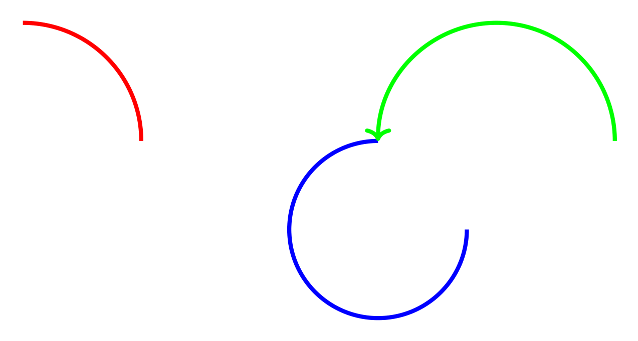
Show the TikZ code
% --------------------------------------------- %% Tikzfigure generated by tikzfigure v0.5.0 %% https://github.com/max-models/tikzfigure %% --------------------------------------------- %\begin{tikzpicture} \draw[color=red, line width=2pt, start angle=0, end angle=90, radius=2cm] ({0}, {0}) arc; \draw[color=blue, line width=2pt, start angle=90, end angle=360, radius=1.5cm] ({4}, {0}) arc; \draw[->, color=green, line width=2pt, start angle=0, end angle=180, radius=2cm] ({8}, {0}) arc;\end{tikzpicture}Show the standalone LaTeX document
\documentclass[border=10pt]{standalone}\PassOptionsToPackage{dvipsnames,svgnames,x11names}{xcolor}\usepackage{tikz}\usepackage{pgfplots}\pgfplotsset{compat=newest}\usepgfplotslibrary{groupplots}\usetikzlibrary{arrows.meta}\begin{document}% --------------------------------------------- %% Tikzfigure generated by tikzfigure v0.5.0     %% https://github.com/max-models/tikzfigure      %% --------------------------------------------- %\begin{tikzpicture}    \draw[color=red, line width=2pt, start angle=0, end angle=90, radius=2cm] ({0}, {0}) arc;    \draw[color=blue, line width=2pt, start angle=90, end angle=360, radius=1.5cm] ({4}, {0}) arc;    \draw[->, color=green, line width=2pt, start angle=0, end angle=180, radius=2cm] ({8}, {0}) arc;\end{tikzpicture}
\end{document}
Circles
Section titled “Circles”A circle is defined by a center point and a radius.
fig = TikzFigure()
# Unfilled circlefig.circle(    center=(0, 0),    radius="1cm",    color="blue",    line_width="2pt",)
# Filled circlefig.circle(    center=(3, 0),    radius="1cm",    fill="yellow",    color="orange",    line_width="2pt",)
# Dashed circlefig.circle(    center=(6, 0),    radius="1cm",    color="purple",    dash_pattern="on 2pt off 2pt",    line_width="2pt",)
fig.show()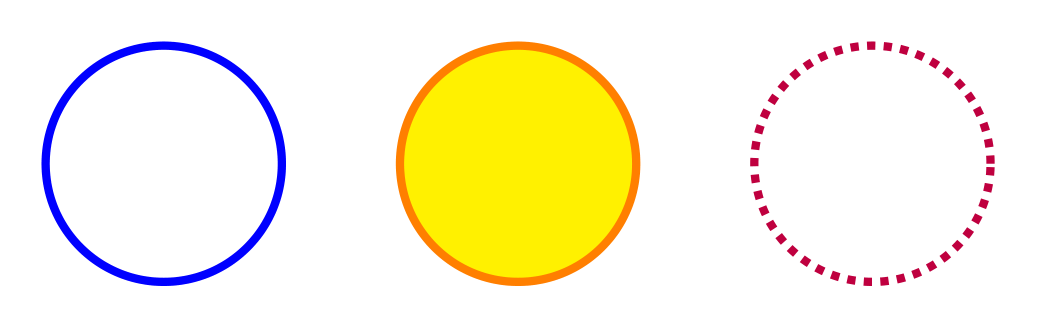
Show the TikZ code
% --------------------------------------------- %% Tikzfigure generated by tikzfigure v0.5.0 %% https://github.com/max-models/tikzfigure %% --------------------------------------------- %\begin{tikzpicture} \draw[color=blue, line width=2pt] ({0}, {0}) circle (1cm); \draw[color=orange, fill=yellow, line width=2pt] ({3}, {0}) circle (1cm); \draw[color=purple, line width=2pt, dash pattern=on 2pt off 2pt] ({6}, {0}) circle (1cm);\end{tikzpicture}Show the standalone LaTeX document
\documentclass[border=10pt]{standalone}\PassOptionsToPackage{dvipsnames,svgnames,x11names}{xcolor}\usepackage{tikz}\usepackage{pgfplots}\pgfplotsset{compat=newest}\usepgfplotslibrary{groupplots}\usetikzlibrary{arrows.meta}\begin{document}% --------------------------------------------- %% Tikzfigure generated by tikzfigure v0.5.0     %% https://github.com/max-models/tikzfigure      %% --------------------------------------------- %\begin{tikzpicture}    \draw[color=blue, line width=2pt] ({0}, {0}) circle (1cm);    \draw[color=orange, fill=yellow, line width=2pt] ({3}, {0}) circle (1cm);    \draw[color=purple, line width=2pt, dash pattern=on 2pt off 2pt] ({6}, {0}) circle (1cm);\end{tikzpicture}
\end{document}
Clock face
Section titled “Clock face”A practical example: a clock face using a circle and line segments for hour markers.
fig = TikzFigure()
# Outer circlefig.circle(    center=(0, 0),    radius="3cm",    color="black",    line_width="2pt",)
# Hour markers (12 arcs around the circle)for hour in range(12):    angle = ((hour + 3) * 30) % 360  # 30 degrees apart    rad = math.radians(angle)
    # Small line segment from inner to outer    x_inner = 2.7 * math.cos(rad)    y_inner = 2.7 * math.sin(rad)    fig.draw(        [(x_inner, y_inner), (x_inner * 1.1, y_inner * 1.1)],        line_width="1.5pt",        color="black",    )
    # Hour numbers    x_text = 2.4 * math.cos(rad)    y_text = 2.4 * math.sin(rad)    fig.node(        x_text,        y_text,        content=str(hour if hour > 0 else 12),        draw="none",    )
# Center dotfig.circle(    center=(0, 0),    radius="0.15cm",    fill="black",)
fig.show()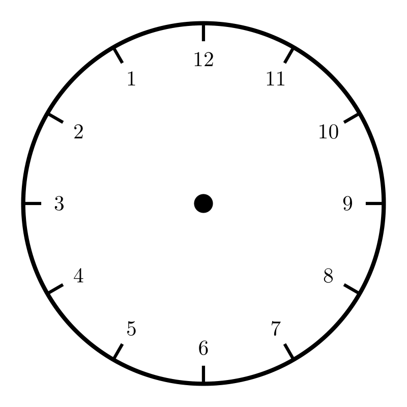
Show the TikZ code
% --------------------------------------------- %% Tikzfigure generated by tikzfigure v0.5.0 %% https://github.com/max-models/tikzfigure %% --------------------------------------------- %\begin{tikzpicture} \draw[color=black, line width=2pt] ({0}, {0}) circle (3cm); \draw[color=black, line width=1.5pt] (1.6532731788489269e-16, 2.7) to (1.8186004967338198e-16, 2.9700000000000006); \node[draw=none] (node0) at ({1.4695761589768238e-16}, {2.4}) {12}; \draw[color=black, line width=1.5pt] (-1.3499999999999994, 2.3382685902179845) to (-1.4849999999999994, 2.572095449239783); \node[draw=none] (node1) at ({-1.1999999999999995}, {2.078460969082653}) {1}; \draw[color=black, line width=1.5pt] (-2.3382685902179845, 1.3499999999999999) to (-2.572095449239783, 1.4849999999999999); \node[draw=none] (node2) at ({-2.078460969082653}, {1.1999999999999997}) {2}; \draw[color=black, line width=1.5pt] (-2.7, 3.3065463576978537e-16) to (-2.9700000000000006, 3.6372009934676396e-16); \node[draw=none] (node3) at ({-2.4}, {2.9391523179536476e-16}) {3}; \draw[color=black, line width=1.5pt] (-2.3382685902179845, -1.3500000000000003) to (-2.572095449239783, -1.4850000000000005); \node[draw=none] (node4) at ({-2.0784609690826525}, {-1.2000000000000002}) {4}; \draw[color=black, line width=1.5pt] (-1.3500000000000012, -2.3382685902179836) to (-1.4850000000000014, -2.5720954492397823); \node[draw=none] (node5) at ({-1.200000000000001}, {-2.078460969082652}) {5}; \draw[color=black, line width=1.5pt] (-4.959819536546781e-16, -2.7) to (-5.455801490201459e-16, -2.9700000000000006); \node[draw=none] (node6) at ({-4.408728476930471e-16}, {-2.4}) {6}; \draw[color=black, line width=1.5pt] (1.3500000000000003, -2.3382685902179845) to (1.4850000000000005, -2.572095449239783); \node[draw=none] (node7) at ({1.2000000000000002}, {-2.0784609690826525}) {7}; \draw[color=black, line width=1.5pt] (2.3382685902179836, -1.3500000000000012) to (2.5720954492397823, -1.4850000000000014); \node[draw=none] (node8) at ({2.078460969082652}, {-1.200000000000001}) {8}; \draw[color=black, line width=1.5pt] (2.7, 0.0) to (2.9700000000000006, 0.0); \node[draw=none] (node9) at ({2.4}, {0.0}) {9}; \draw[color=black, line width=1.5pt] (2.3382685902179845, 1.3499999999999999) to (2.572095449239783, 1.4849999999999999); \node[draw=none] (node10) at ({2.078460969082653}, {1.1999999999999997}) {10}; \draw[color=black, line width=1.5pt] (1.3500000000000003, 2.3382685902179845) to (1.4850000000000005, 2.572095449239783); \node[draw=none] (node11) at ({1.2000000000000002}, {2.0784609690826525}) {11}; \draw[fill=black] ({0}, {0}) circle (0.15cm);\end{tikzpicture}Show the standalone LaTeX document
\documentclass[border=10pt]{standalone}\PassOptionsToPackage{dvipsnames,svgnames,x11names}{xcolor}\usepackage{tikz}\usepackage{pgfplots}\pgfplotsset{compat=newest}\usepgfplotslibrary{groupplots}\usetikzlibrary{arrows.meta}\begin{document}% --------------------------------------------- %% Tikzfigure generated by tikzfigure v0.5.0     %% https://github.com/max-models/tikzfigure      %% --------------------------------------------- %\begin{tikzpicture}    \draw[color=black, line width=2pt] ({0}, {0}) circle (3cm);    \draw[color=black, line width=1.5pt] (1.6532731788489269e-16, 2.7) to (1.8186004967338198e-16, 2.9700000000000006);    \node[draw=none] (node0) at ({1.4695761589768238e-16}, {2.4}) {12};    \draw[color=black, line width=1.5pt] (-1.3499999999999994, 2.3382685902179845) to (-1.4849999999999994, 2.572095449239783);    \node[draw=none] (node1) at ({-1.1999999999999995}, {2.078460969082653}) {1};    \draw[color=black, line width=1.5pt] (-2.3382685902179845, 1.3499999999999999) to (-2.572095449239783, 1.4849999999999999);    \node[draw=none] (node2) at ({-2.078460969082653}, {1.1999999999999997}) {2};    \draw[color=black, line width=1.5pt] (-2.7, 3.3065463576978537e-16) to (-2.9700000000000006, 3.6372009934676396e-16);    \node[draw=none] (node3) at ({-2.4}, {2.9391523179536476e-16}) {3};    \draw[color=black, line width=1.5pt] (-2.3382685902179845, -1.3500000000000003) to (-2.572095449239783, -1.4850000000000005);    \node[draw=none] (node4) at ({-2.0784609690826525}, {-1.2000000000000002}) {4};    \draw[color=black, line width=1.5pt] (-1.3500000000000012, -2.3382685902179836) to (-1.4850000000000014, -2.5720954492397823);    \node[draw=none] (node5) at ({-1.200000000000001}, {-2.078460969082652}) {5};    \draw[color=black, line width=1.5pt] (-4.959819536546781e-16, -2.7) to (-5.455801490201459e-16, -2.9700000000000006);    \node[draw=none] (node6) at ({-4.408728476930471e-16}, {-2.4}) {6};    \draw[color=black, line width=1.5pt] (1.3500000000000003, -2.3382685902179845) to (1.4850000000000005, -2.572095449239783);    \node[draw=none] (node7) at ({1.2000000000000002}, {-2.0784609690826525}) {7};    \draw[color=black, line width=1.5pt] (2.3382685902179836, -1.3500000000000012) to (2.5720954492397823, -1.4850000000000014);    \node[draw=none] (node8) at ({2.078460969082652}, {-1.200000000000001}) {8};    \draw[color=black, line width=1.5pt] (2.7, 0.0) to (2.9700000000000006, 0.0);    \node[draw=none] (node9) at ({2.4}, {0.0}) {9};    \draw[color=black, line width=1.5pt] (2.3382685902179845, 1.3499999999999999) to (2.572095449239783, 1.4849999999999999);    \node[draw=none] (node10) at ({2.078460969082653}, {1.1999999999999997}) {10};    \draw[color=black, line width=1.5pt] (1.3500000000000003, 2.3382685902179845) to (1.4850000000000005, 2.572095449239783);    \node[draw=none] (node11) at ({1.2000000000000002}, {2.0784609690826525}) {11};    \draw[fill=black] ({0}, {0}) circle (0.15cm);\end{tikzpicture}
\end{document}
Rectangles
Section titled “Rectangles”Rectangles are defined by two opposite corners.
fig = TikzFigure()
# Unfilled rectanglefig.rectangle(    (0, 0),    (2, 1),    color="blue",    line_width="2pt",)
# Filled rectanglefig.rectangle(    (3, 0),    (5, 1),    fill="yellow",    color="orange",    line_width="2pt",)
# Rectangle with rounded cornersfig.rectangle(    (6, 0),    (8, 1),    fill="green!30",    color="green",    rounded_corners="5pt",    line_width="2pt",)
fig.show()
Show the TikZ code
% --------------------------------------------- %% Tikzfigure generated by tikzfigure v0.5.0 %% https://github.com/max-models/tikzfigure %% --------------------------------------------- %\begin{tikzpicture} \draw[color=blue, line width=2pt] ({0}, {0}) rectangle ({2}, {1}); \draw[color=orange, fill=yellow, line width=2pt] ({3}, {0}) rectangle ({5}, {1}); \draw[color=green, fill=green!30, line width=2pt, rounded corners=5pt] ({6}, {0}) rectangle ({8}, {1});\end{tikzpicture}Show the standalone LaTeX document
\documentclass[border=10pt]{standalone}\PassOptionsToPackage{dvipsnames,svgnames,x11names}{xcolor}\usepackage{tikz}\usepackage{pgfplots}\pgfplotsset{compat=newest}\usepgfplotslibrary{groupplots}\usetikzlibrary{arrows.meta}\begin{document}% --------------------------------------------- %% Tikzfigure generated by tikzfigure v0.5.0     %% https://github.com/max-models/tikzfigure      %% --------------------------------------------- %\begin{tikzpicture}    \draw[color=blue, line width=2pt] ({0}, {0}) rectangle ({2}, {1});    \draw[color=orange, fill=yellow, line width=2pt] ({3}, {0}) rectangle ({5}, {1});    \draw[color=green, fill=green!30, line width=2pt, rounded corners=5pt] ({6}, {0}) rectangle ({8}, {1});\end{tikzpicture}
\end{document}
Ellipses
Section titled “Ellipses”Ellipses are defined by a center point and two radii.
fig = TikzFigure()
# Circle (equal radii)fig.ellipse(    (0, 0),    x_radius="1cm",    y_radius="1cm",    color="red",    line_width="2pt",)
# Horizontal ellipsefig.ellipse(    (4, 0),    x_radius="1.5cm",    y_radius="0.75cm",    color="blue",    line_width="2pt",)
# Filled ellipsefig.ellipse(    (8, 0),    x_radius="1.2cm",    y_radius="0.8cm",    fill="purple!40",    color="purple",    line_width="2pt",)
fig.show()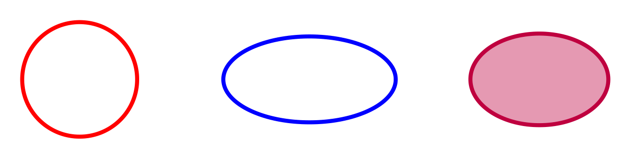
Show the TikZ code
% --------------------------------------------- %% Tikzfigure generated by tikzfigure v0.5.0 %% https://github.com/max-models/tikzfigure %% --------------------------------------------- %\begin{tikzpicture} \draw[color=red, line width=2pt] ({0}, {0}) ellipse (1cm and 1cm); \draw[color=blue, line width=2pt] ({4}, {0}) ellipse (1.5cm and 0.75cm); \draw[color=purple, fill=purple!40, line width=2pt] ({8}, {0}) ellipse (1.2cm and 0.8cm);\end{tikzpicture}Show the standalone LaTeX document
\documentclass[border=10pt]{standalone}\PassOptionsToPackage{dvipsnames,svgnames,x11names}{xcolor}\usepackage{tikz}\usepackage{pgfplots}\pgfplotsset{compat=newest}\usepgfplotslibrary{groupplots}\usetikzlibrary{arrows.meta}\begin{document}% --------------------------------------------- %% Tikzfigure generated by tikzfigure v0.5.0     %% https://github.com/max-models/tikzfigure      %% --------------------------------------------- %\begin{tikzpicture}    \draw[color=red, line width=2pt] ({0}, {0}) ellipse (1cm and 1cm);    \draw[color=blue, line width=2pt] ({4}, {0}) ellipse (1.5cm and 0.75cm);    \draw[color=purple, fill=purple!40, line width=2pt] ({8}, {0}) ellipse (1.2cm and 0.8cm);\end{tikzpicture}
\end{document}A grid spans between two opposite corners with a specified step size.
fig = TikzFigure()
# Uniform gridfig.grid(    (0, 0),    (3, 3),    step="0.5cm",    color="gray!30",)
# Grid with different x and y stepsfig.grid(    (4, 0),    (7, 3),    xstep="0.5cm",    ystep="1cm",    color="blue!20",)
# Grid with larger stepfig.grid(    (8, 0),    (10, 3),    step="1cm",    color="red!20",    line_width="1pt",)
fig.show()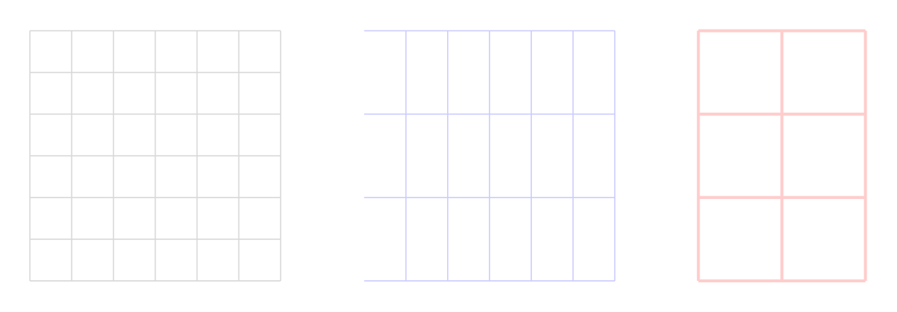
Show the TikZ code
% --------------------------------------------- %% Tikzfigure generated by tikzfigure v0.5.0 %% https://github.com/max-models/tikzfigure %% --------------------------------------------- %\begin{tikzpicture} \draw[color=gray!30, step=0.5cm] ({0}, {0}) grid ({3}, {3}); \draw[color=blue!20, xstep=0.5cm, ystep=1cm] ({4}, {0}) grid ({7}, {3}); \draw[color=red!20, line width=1pt, step=1cm] ({8}, {0}) grid ({10}, {3});\end{tikzpicture}Show the standalone LaTeX document
\documentclass[border=10pt]{standalone}\PassOptionsToPackage{dvipsnames,svgnames,x11names}{xcolor}\usepackage{tikz}\usepackage{pgfplots}\pgfplotsset{compat=newest}\usepgfplotslibrary{groupplots}\usetikzlibrary{arrows.meta}\begin{document}% --------------------------------------------- %% Tikzfigure generated by tikzfigure v0.5.0     %% https://github.com/max-models/tikzfigure      %% --------------------------------------------- %\begin{tikzpicture}    \draw[color=gray!30, step=0.5cm] ({0}, {0}) grid ({3}, {3});    \draw[color=blue!20, xstep=0.5cm, ystep=1cm] ({4}, {0}) grid ({7}, {3});    \draw[color=red!20, line width=1pt, step=1cm] ({8}, {0}) grid ({10}, {3});\end{tikzpicture}
\end{document}
Parabolas
Section titled “Parabolas”Parabolas connect two points, optionally with a bend (control) point.
fig = TikzFigure()
# Simple parabolafig.parabola(    (0, 0),    (3, 0),    color="red",    line_width="2pt",)
# Parabola with bend point (creates a specific curve shape)fig.parabola(    (5, 0),    (8, 0),    bend=(6.5, 2),    color="blue",    line_width="2pt",)
# Parabola with arrowfig.parabola(    (0, 3),    (3, 4),    color="green",    arrows=arrows.forward,    line_width="2pt",)
fig.show()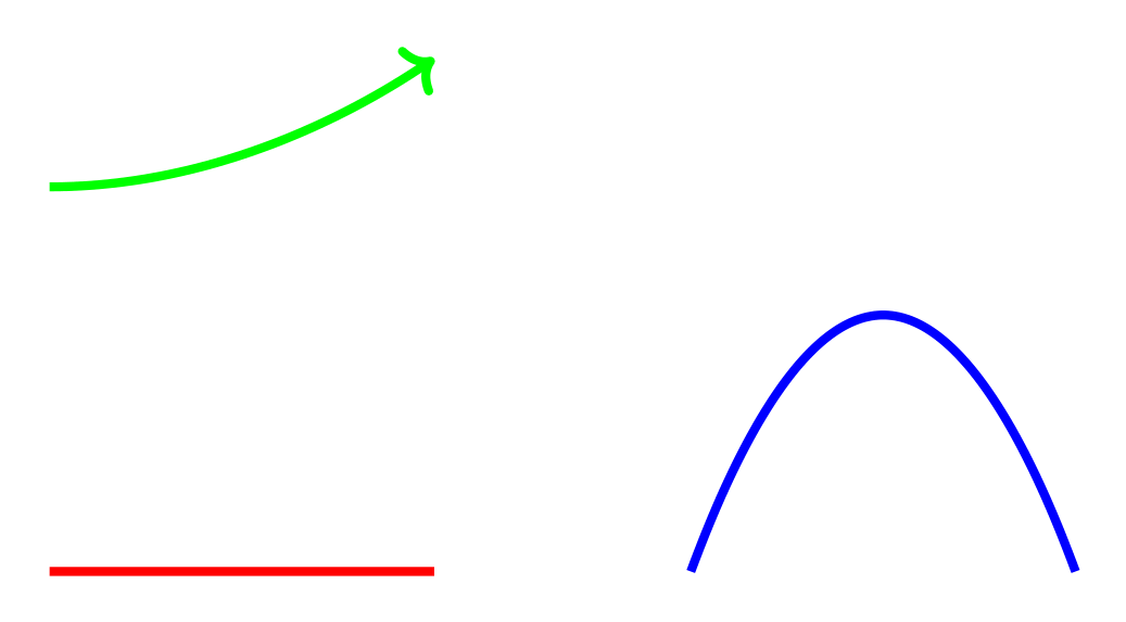
Show the TikZ code
% --------------------------------------------- %% Tikzfigure generated by tikzfigure v0.5.0 %% https://github.com/max-models/tikzfigure %% --------------------------------------------- %\begin{tikzpicture} \draw[color=red, line width=2pt] ({0}, {0}) parabola ({3}, {0}); \draw[color=blue, line width=2pt] ({5}, {0}) parabola bend ({6.5}, {2}) ({8}, {0}); \draw[->, color=green, line width=2pt] ({0}, {3}) parabola ({3}, {4});\end{tikzpicture}Show the standalone LaTeX document
\documentclass[border=10pt]{standalone}\PassOptionsToPackage{dvipsnames,svgnames,x11names}{xcolor}\usepackage{tikz}\usepackage{pgfplots}\pgfplotsset{compat=newest}\usepgfplotslibrary{groupplots}\usetikzlibrary{arrows.meta}\begin{document}% --------------------------------------------- %% Tikzfigure generated by tikzfigure v0.5.0     %% https://github.com/max-models/tikzfigure      %% --------------------------------------------- %\begin{tikzpicture}    \draw[color=red, line width=2pt] ({0}, {0}) parabola ({3}, {0});    \draw[color=blue, line width=2pt] ({5}, {0}) parabola bend ({6.5}, {2}) ({8}, {0});    \draw[->, color=green, line width=2pt] ({0}, {3}) parabola ({3}, {4});\end{tikzpicture}
\end{document}
Lines and intersections
Section titled “Lines and intersections”Lines connect two points and support arrows and all standard styling.
fig = TikzFigure()
# Simple linefig.line(    (0, 0),    (2, 0),    color="red",    line_width="2pt",)
# Line with arrowfig.line(    (3, 0),    (5, 2),    color="blue",    arrows=arrows.forward,    line_width="2pt",)
# Dashed linefig.line(    (6, 0),    (8, 1),    color="green",    options=[styles.dashed],    line_width="2pt",)
fig.show()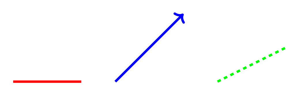
Show the TikZ code
% --------------------------------------------- %% Tikzfigure generated by tikzfigure v0.5.0 %% https://github.com/max-models/tikzfigure %% --------------------------------------------- %\begin{tikzpicture} \draw[color=red, line width=2pt] ({0}, {0}) -- ({2}, {0}); \draw[->, color=blue, line width=2pt] ({3}, {0}) -- ({5}, {2}); \draw[dashed, color=green, line width=2pt] ({6}, {0}) -- ({8}, {1});\end{tikzpicture}Show the standalone LaTeX document
\documentclass[border=10pt]{standalone}\PassOptionsToPackage{dvipsnames,svgnames,x11names}{xcolor}\usepackage{tikz}\usepackage{pgfplots}\pgfplotsset{compat=newest}\usepgfplotslibrary{groupplots}\usetikzlibrary{arrows.meta}\begin{document}% --------------------------------------------- %% Tikzfigure generated by tikzfigure v0.5.0     %% https://github.com/max-models/tikzfigure      %% --------------------------------------------- %\begin{tikzpicture}    \draw[color=red, line width=2pt] ({0}, {0}) -- ({2}, {0});    \draw[->, color=blue, line width=2pt] ({3}, {0}) -- ({5}, {2});    \draw[dashed, color=green, line width=2pt] ({6}, {0}) -- ({8}, {1});\end{tikzpicture}
\end{document}
Find where two lines intersect using the intersection() method:
fig = TikzFigure()

# Create two linesline1 = fig.line(    (0, 0),    (4, 4),    color="red",    line_width="2pt",)line2 = fig.line(    (0, 4),    (4, 0),    color="blue",    line_width="2pt",)
# Find intersectionintersection = line1.intersection(line2)print(f"Lines intersect at: {intersection}")
# Draw intersection pointif intersection:    fig.node(        intersection[0],        intersection[1],        shape="circle",        fill="black",        minimum_size="0.15cm",        draw="none",    )
fig.show()
Lines intersect at: (2.0, 2.0)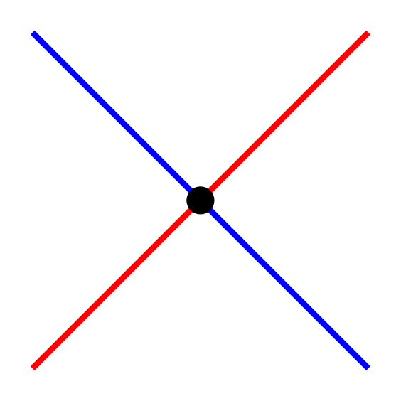
Show the TikZ code
% --------------------------------------------- %% Tikzfigure generated by tikzfigure v0.5.0 %% https://github.com/max-models/tikzfigure %% --------------------------------------------- %\begin{tikzpicture} \draw[color=red, line width=2pt] ({0}, {0}) -- ({4}, {4}); \draw[color=blue, line width=2pt] ({0}, {4}) -- ({4}, {0}); \node[shape=circle, fill=black, draw=none, minimum size=0.15cm] (node0) at ({2.0}, {2.0}) {};\end{tikzpicture}Show the standalone LaTeX document
\documentclass[border=10pt]{standalone}\PassOptionsToPackage{dvipsnames,svgnames,x11names}{xcolor}\usepackage{tikz}\usepackage{pgfplots}\pgfplotsset{compat=newest}\usepgfplotslibrary{groupplots}\usetikzlibrary{arrows.meta}\begin{document}% --------------------------------------------- %% Tikzfigure generated by tikzfigure v0.5.0     %% https://github.com/max-models/tikzfigure      %% --------------------------------------------- %\begin{tikzpicture}    \draw[color=red, line width=2pt] ({0}, {0}) -- ({4}, {4});    \draw[color=blue, line width=2pt] ({0}, {4}) -- ({4}, {0});    \node[shape=circle, fill=black, draw=none, minimum size=0.15cm] (node0) at ({2.0}, {2.0}) {};\end{tikzpicture}
\end{document}
Regular polygons
Section titled “Regular polygons”Draw regular polygons (triangle, square, pentagon, etc.) with specified center and radius.
fig = TikzFigure()
# Triangle (3 sides)fig.triangle(    (0, 1),    radius=0.8,    color="red",    fill="red!20",)
# Square (4 sides)fig.square(    (3, 1),    radius=0.8,    color="blue",    fill="blue!20",)
# Pentagon (5 sides)fig.polygon(    (6, 1),    radius=0.8,    sides=5,    color="green",    fill="green!20",)
# Hexagon (6 sides)fig.polygon(    (9, 1),    radius=0.8,    sides=6,    color="orange",    fill="orange!20",)
fig.show()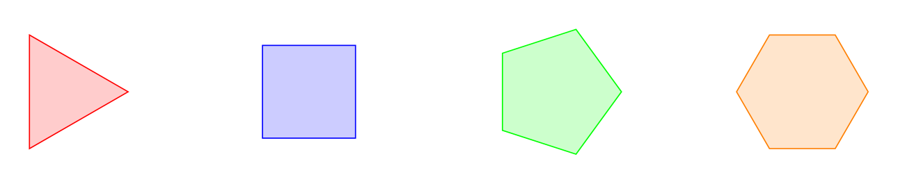
Show the TikZ code
% --------------------------------------------- %% Tikzfigure generated by tikzfigure v0.5.0 %% https://github.com/max-models/tikzfigure %% --------------------------------------------- %\begin{tikzpicture} \draw[color=red, fill=red!20] (0.8, 1.0) -- (-0.4, 1.692820323028) -- (-0.4, 0.307179676972) -- cycle; \draw[color=blue, fill=blue!20] (3.565685424949, 1.565685424949) -- (2.434314575051, 1.565685424949) -- (2.434314575051, 0.434314575051) -- (3.565685424949, 0.434314575051) -- cycle; \draw[color=green, fill=green!20] (6.8, 1.0) -- (6.2472135955, 1.760845213036) -- (5.3527864045, 1.470228201834) -- (5.3527864045, 0.529771798166) -- (6.2472135955, 0.239154786964) -- cycle; \draw[color=orange, fill=orange!20] (9.8, 1.0) -- (9.4, 1.692820323028) -- (8.6, 1.692820323028) -- (8.2, 1.0) -- (8.6, 0.307179676972) -- (9.4, 0.307179676972) -- cycle;\end{tikzpicture}Show the standalone LaTeX document
\documentclass[border=10pt]{standalone}\PassOptionsToPackage{dvipsnames,svgnames,x11names}{xcolor}\usepackage{tikz}\usepackage{pgfplots}\pgfplotsset{compat=newest}\usepgfplotslibrary{groupplots}\usetikzlibrary{arrows.meta}\begin{document}% --------------------------------------------- %% Tikzfigure generated by tikzfigure v0.5.0     %% https://github.com/max-models/tikzfigure      %% --------------------------------------------- %\begin{tikzpicture}    \draw[color=red, fill=red!20] (0.8, 1.0) -- (-0.4, 1.692820323028) -- (-0.4, 0.307179676972) -- cycle;    \draw[color=blue, fill=blue!20] (3.565685424949, 1.565685424949) -- (2.434314575051, 1.565685424949) -- (2.434314575051, 0.434314575051) -- (3.565685424949, 0.434314575051) -- cycle;    \draw[color=green, fill=green!20] (6.8, 1.0) -- (6.2472135955, 1.760845213036) -- (5.3527864045, 1.470228201834) -- (5.3527864045, 0.529771798166) -- (6.2472135955, 0.239154786964) -- cycle;    \draw[color=orange, fill=orange!20] (9.8, 1.0) -- (9.4, 1.692820323028) -- (8.6, 1.692820323028) -- (8.2, 1.0) -- (8.6, 0.307179676972) -- (9.4, 0.307179676972) -- cycle;\end{tikzpicture}
\end{document}
Rotated polygons
Section titled “Rotated polygons”Polygons can be rotated by specifying a rotation angle in degrees.
fig = TikzFigure()
# Squares with different rotationsrotations = [0, 22.5, 45]for i, rot in enumerate(rotations):    fig.square(        (i * 3, 1),        radius=0.8,        rotation=rot,        color="purple",        fill="purple!30",    )    fig.node(        i * 3,        -0.3,        content=f"{rot}\\textdegree",        draw="none",    )
# Triangles pointing in different directionsfig.triangle(    (0, 3.5),    radius=0.8,    rotation=0,    color="blue",    fill="blue!20",)fig.triangle(    (3, 3.5),    radius=0.8,    rotation=120,    color="blue",    fill="blue!20",)fig.triangle(    (6, 3.5),    radius=0.8,    rotation=240,    color="blue",    fill="blue!20",)
fig.show()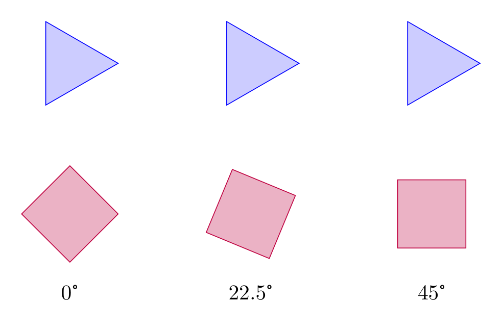
Show the TikZ code
% --------------------------------------------- %% Tikzfigure generated by tikzfigure v0.5.0 %% https://github.com/max-models/tikzfigure %% --------------------------------------------- %\begin{tikzpicture} \draw[color=purple, fill=purple!30] (0.8, 1.0) -- (0.0, 1.8) -- (-0.8, 1.0) -- (-0.0, 0.2) -- cycle; \node[draw=none] (node0) at ({0}, {-0.3}) {0\textdegree}; \draw[color=purple, fill=purple!30] (3.739103626009, 1.306146745892) -- (2.693853254108, 1.739103626009) -- (2.260896373991, 0.693853254108) -- (3.306146745892, 0.260896373991) -- cycle; \node[draw=none] (node1) at ({3}, {-0.3}) {22.5\textdegree}; \draw[color=purple, fill=purple!30] (6.565685424949, 1.565685424949) -- (5.434314575051, 1.565685424949) -- (5.434314575051, 0.434314575051) -- (6.565685424949, 0.434314575051) -- cycle; \node[draw=none] (node2) at ({6}, {-0.3}) {45\textdegree}; \draw[color=blue, fill=blue!20] (0.8, 3.5) -- (-0.4, 4.192820323028) -- (-0.4, 2.807179676972) -- cycle; \draw[color=blue, fill=blue!20] (2.6, 4.192820323028) -- (2.6, 2.807179676972) -- (3.8, 3.5) -- cycle; \draw[color=blue, fill=blue!20] (5.6, 2.807179676972) -- (6.8, 3.5) -- (5.6, 4.192820323028) -- cycle;\end{tikzpicture}Show the standalone LaTeX document
\documentclass[border=10pt]{standalone}\PassOptionsToPackage{dvipsnames,svgnames,x11names}{xcolor}\usepackage{tikz}\usepackage{pgfplots}\pgfplotsset{compat=newest}\usepgfplotslibrary{groupplots}\usetikzlibrary{arrows.meta}\begin{document}% --------------------------------------------- %% Tikzfigure generated by tikzfigure v0.5.0     %% https://github.com/max-models/tikzfigure      %% --------------------------------------------- %\begin{tikzpicture}    \draw[color=purple, fill=purple!30] (0.8, 1.0) -- (0.0, 1.8) -- (-0.8, 1.0) -- (-0.0, 0.2) -- cycle;    \node[draw=none] (node0) at ({0}, {-0.3}) {0\textdegree};    \draw[color=purple, fill=purple!30] (3.739103626009, 1.306146745892) -- (2.693853254108, 1.739103626009) -- (2.260896373991, 0.693853254108) -- (3.306146745892, 0.260896373991) -- cycle;    \node[draw=none] (node1) at ({3}, {-0.3}) {22.5\textdegree};    \draw[color=purple, fill=purple!30] (6.565685424949, 1.565685424949) -- (5.434314575051, 1.565685424949) -- (5.434314575051, 0.434314575051) -- (6.565685424949, 0.434314575051) -- cycle;    \node[draw=none] (node2) at ({6}, {-0.3}) {45\textdegree};    \draw[color=blue, fill=blue!20] (0.8, 3.5) -- (-0.4, 4.192820323028) -- (-0.4, 2.807179676972) -- cycle;    \draw[color=blue, fill=blue!20] (2.6, 4.192820323028) -- (2.6, 2.807179676972) -- (3.8, 3.5) -- cycle;    \draw[color=blue, fill=blue!20] (5.6, 2.807179676972) -- (6.8, 3.5) -- (5.6, 4.192820323028) -- cycle;\end{tikzpicture}
\end{document}
Matrix of nodes
Section titled “Matrix of nodes”add_matrix() lays out a grid of nodes using TikZ’s matrix library, so you
don’t need to hand-write raw \matrix code. Cells are given row by row, and
per-cell styling is set with a {"content": ..., **options} dict. Use
row_sep, column_sep, and cell_style to control spacing and the shared
look of every cell.
fig = TikzFigure()
fig.add_matrix(    [        ["A", "B", "C"],        ["D", {"content": "E", "fill": "yellow!60"}, "F"],    ],    label="grid",    options="matrix of nodes",    row_sep="5pt",    column_sep="5pt",    cell_style="draw, minimum size=1cm, anchor=center",)
fig.show()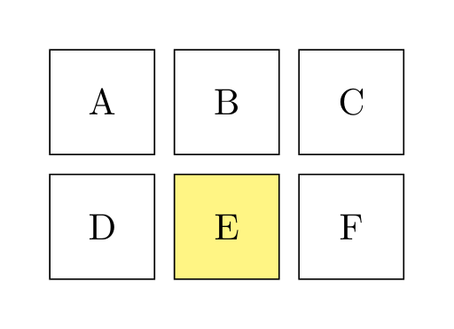
Show the TikZ code
% --------------------------------------------- %% Tikzfigure generated by tikzfigure v0.5.0 %% https://github.com/max-models/tikzfigure %% --------------------------------------------- %\begin{tikzpicture} \matrix[matrix of nodes, nodes={draw, minimum size=1cm, anchor=center}, row sep=5pt, column sep=5pt] (grid) { A & B & C \\ D & |[fill=yellow!60]| E & F \\ };\end{tikzpicture}Show the standalone LaTeX document
\documentclass[border=10pt]{standalone}\PassOptionsToPackage{dvipsnames,svgnames,x11names}{xcolor}\usepackage{tikz}\usepackage{pgfplots}\pgfplotsset{compat=newest}\usepgfplotslibrary{groupplots}\usetikzlibrary{arrows.meta,matrix}\begin{document}% --------------------------------------------- %% Tikzfigure generated by tikzfigure v0.5.0     %% https://github.com/max-models/tikzfigure      %% --------------------------------------------- %\begin{tikzpicture}    \matrix[matrix of nodes, nodes={draw, minimum size=1cm, anchor=center}, row sep=5pt, column sep=5pt] (grid) {      A & B & C \\      D & |[fill=yellow!60]| E & F \\    };\end{tikzpicture}
\end{document}
Individual cells are addressable with Matrix.cell(row, col), which returns
the TikZ node name for that cell ("<label>-<row>-<col>", 1-indexed). Turn
that name into a figure coordinate with add_coordinate(..., at=...) to draw
connections between cells:
fig = TikzFigure()
grid = fig.add_matrix(    [["A", "B"], ["C", "D"]],    label="grid",    options="matrix of nodes",    row_sep="5pt",    column_sep="5pt",    cell_style="draw, minimum size=1cm, anchor=center",)
fig.add_coordinate("c1", at=grid.cell(1, 1))fig.add_coordinate("c2", at=grid.cell(2, 2))fig.draw(["c1", "c2"], arrows=arrows.forward, color="red", line_width="1.5pt")
fig.show()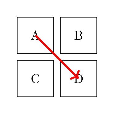
Show the TikZ code
% --------------------------------------------- %% Tikzfigure generated by tikzfigure v0.5.0 %% https://github.com/max-models/tikzfigure %% --------------------------------------------- %\begin{tikzpicture} \matrix[matrix of nodes, nodes={draw, minimum size=1cm, anchor=center}, row sep=5pt, column sep=5pt] (grid) { A & B \\ C & D \\ }; \coordinate (c1) at (grid-1-1); \coordinate (c2) at (grid-2-2); \draw[->, color=red, line width=1.5pt] (c1) to (c2);\end{tikzpicture}Show the standalone LaTeX document
\documentclass[border=10pt]{standalone}\PassOptionsToPackage{dvipsnames,svgnames,x11names}{xcolor}\usepackage{tikz}\usepackage{pgfplots}\pgfplotsset{compat=newest}\usepgfplotslibrary{groupplots}\usetikzlibrary{arrows.meta,matrix}\begin{document}% --------------------------------------------- %% Tikzfigure generated by tikzfigure v0.5.0     %% https://github.com/max-models/tikzfigure      %% --------------------------------------------- %\begin{tikzpicture}    \matrix[matrix of nodes, nodes={draw, minimum size=1cm, anchor=center}, row sep=5pt, column sep=5pt] (grid) {      A & B \\      C & D \\    };    \coordinate (c1) at (grid-1-1);    \coordinate (c2) at (grid-2-2);    \draw[->, color=red, line width=1.5pt] (c1) to (c2);\end{tikzpicture}
\end{document}
Matrix.arrow(source, target, label=...) draws an arrow between two cells,
from border to border, with an optional label node. Cells are (row, col) tuples
(1-indexed) or any node name, such as a cell of another matrix. With
options="matrix of math nodes" this gives commutative diagrams:
fig = TikzFigure()
diagram = fig.add_matrix(    [["V^0", "V^1", "V^2"], ["H^1", r"H(\mathrm{curl})", "L^2"]],    label="d",    options="matrix of math nodes",    row_sep="1.2cm",    column_sep="1.6cm",    cell_style="text height=1.5ex, text depth=0.25ex",)
for row in (1, 2):    diagram.arrow((row, 1), (row, 2), label=r"$\nabla$")    diagram.arrow((row, 2), (row, 3), label=r"$\nabla\times$")for col in (1, 2, 3):    diagram.arrow(        (2, col),        (1, col),        label=rf"$\pi^{col - 1}$",        label_position="left",        color="blue",    )
fig.show()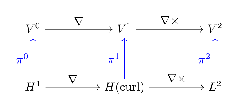
Show the TikZ code
% --------------------------------------------- %% Tikzfigure generated by tikzfigure v0.5.0 %% https://github.com/max-models/tikzfigure %% --------------------------------------------- %\begin{tikzpicture} \matrix[matrix of math nodes, nodes={text height=1.5ex, text depth=0.25ex}, row sep=1.2cm, column sep=1.6cm] (d) { V^0 & V^1 & V^2 \\ H^1 & H(\mathrm{curl}) & L^2 \\ }; \draw[->] (d-1-1) to node[above] {$\nabla$} (d-1-2); \draw[->] (d-1-2) to node[above] {$\nabla\times$} (d-1-3); \draw[->] (d-2-1) to node[above] {$\nabla$} (d-2-2); \draw[->] (d-2-2) to node[above] {$\nabla\times$} (d-2-3); \draw[->, color=blue] (d-2-1) to node[left] {$\pi^0$} (d-1-1); \draw[->, color=blue] (d-2-2) to node[left] {$\pi^1$} (d-1-2); \draw[->, color=blue] (d-2-3) to node[left] {$\pi^2$} (d-1-3);\end{tikzpicture}Show the standalone LaTeX document
\documentclass[border=10pt]{standalone}\PassOptionsToPackage{dvipsnames,svgnames,x11names}{xcolor}\usepackage{tikz}\usepackage{pgfplots}\pgfplotsset{compat=newest}\usepgfplotslibrary{groupplots}\usetikzlibrary{arrows.meta,matrix}\begin{document}% --------------------------------------------- %% Tikzfigure generated by tikzfigure v0.5.0     %% https://github.com/max-models/tikzfigure      %% --------------------------------------------- %\begin{tikzpicture}    \matrix[matrix of math nodes, nodes={text height=1.5ex, text depth=0.25ex}, row sep=1.2cm, column sep=1.6cm] (d) {      V^0 & V^1 & V^2 \\      H^1 & H(\mathrm{curl}) & L^2 \\    };    \draw[->] (d-1-1) to node[above] {$\nabla$} (d-1-2);    \draw[->] (d-1-2) to node[above] {$\nabla\times$} (d-1-3);    \draw[->] (d-2-1) to node[above] {$\nabla$} (d-2-2);    \draw[->] (d-2-2) to node[above] {$\nabla\times$} (d-2-3);    \draw[->, color=blue] (d-2-1) to node[left] {$\pi^0$} (d-1-1);    \draw[->, color=blue] (d-2-2) to node[left] {$\pi^1$} (d-1-2);    \draw[->, color=blue] (d-2-3) to node[left] {$\pi^2$} (d-1-3);\end{tikzpicture}
\end{document}
Fit boxes around nodes
Section titled “Fit boxes around nodes”add_fit() wraps a group of existing nodes/coordinates in a single bounding
node, using TikZ’s fit library - handy for drawing a background box around
related elements without hand-writing fit=(...).... Pass the Node/
Coordinate objects (or their label strings) to fit around.
fig = TikzFigure()
a = fig.node((0, 0), shape="circle", fill="blue!30", content="A")b = fig.node((3, 0), shape="circle", fill="blue!30", content="B")c = fig.node((1.5, 2), shape="circle", fill="blue!30", content="C")
fig.add_fit(    [a, b, c],    options=["draw", "dashed", "rounded corners"],    inner_sep="0.4cm",)
fig.show()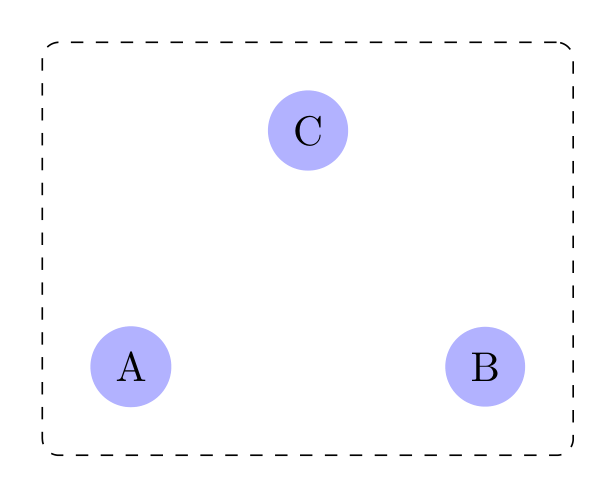
Show the TikZ code
% --------------------------------------------- %% Tikzfigure generated by tikzfigure v0.5.0 %% https://github.com/max-models/tikzfigure %% --------------------------------------------- %\begin{tikzpicture} \node[shape=circle, fill=blue!30] (node0) at ({0}, {0}) {A}; \node[shape=circle, fill=blue!30] (node1) at ({3}, {0}) {B}; \node[shape=circle, fill=blue!30] (node2) at ({1.5}, {2}) {C}; \node[fit=(node0)(node1)(node2), draw, dashed, rounded corners, inner sep=0.4cm] (node3) {};\end{tikzpicture}Show the standalone LaTeX document
\documentclass[border=10pt]{standalone}\PassOptionsToPackage{dvipsnames,svgnames,x11names}{xcolor}\usepackage{tikz}\usepackage{pgfplots}\pgfplotsset{compat=newest}\usepgfplotslibrary{groupplots}\usetikzlibrary{arrows.meta,fit}\begin{document}% --------------------------------------------- %% Tikzfigure generated by tikzfigure v0.5.0     %% https://github.com/max-models/tikzfigure      %% --------------------------------------------- %\begin{tikzpicture}    \node[shape=circle, fill=blue!30] (node0) at ({0}, {0}) {A};    \node[shape=circle, fill=blue!30] (node1) at ({3}, {0}) {B};    \node[shape=circle, fill=blue!30] (node2) at ({1.5}, {2}) {C};    \node[fit=(node0)(node1)(node2), draw, dashed, rounded corners, inner sep=0.4cm] (node3) {};\end{tikzpicture}
\end{document}
Fit nodes can be styled like any other node (fill, color, …) and, since
add_fit() returns a regular Node-like object, a title can be placed above
it at an absolute coordinate:
fig = TikzFigure()
x = fig.node((0, 0), content="x")y = fig.node((2, 0), content="y")z = fig.node((1, 1.5), content="z")
fig.add_fit(    [x, y, z],    label="group",    options=["draw"],    color="orange!60",    fill="orange!10",    inner_sep="0.3cm",)fig.node((1, 2.3), content="\\textbf{Group}", draw="none")
fig.show()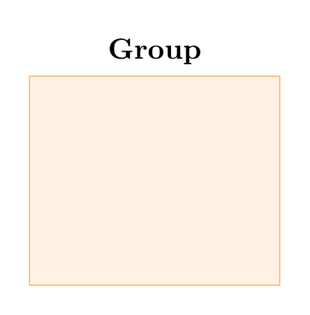
Show the TikZ code
% --------------------------------------------- %% Tikzfigure generated by tikzfigure v0.5.0 %% https://github.com/max-models/tikzfigure %% --------------------------------------------- %\begin{tikzpicture} \node (node0) at ({0}, {0}) {x}; \node (node1) at ({2}, {0}) {y}; \node (node2) at ({1}, {1.5}) {z}; \node[fit=(node0)(node1)(node2), draw, color=orange!60, fill=orange!10, inner sep=0.3cm] (group) {}; \node[draw=none] (node3) at ({1}, {2.3}) {\textbf{Group}};\end{tikzpicture}Show the standalone LaTeX document
\documentclass[border=10pt]{standalone}\PassOptionsToPackage{dvipsnames,svgnames,x11names}{xcolor}\usepackage{tikz}\usepackage{pgfplots}\pgfplotsset{compat=newest}\usepgfplotslibrary{groupplots}\usetikzlibrary{arrows.meta,fit}\begin{document}% --------------------------------------------- %% Tikzfigure generated by tikzfigure v0.5.0     %% https://github.com/max-models/tikzfigure      %% --------------------------------------------- %\begin{tikzpicture}    \node (node0) at ({0}, {0}) {x};    \node (node1) at ({2}, {0}) {y};    \node (node2) at ({1}, {1.5}) {z};    \node[fit=(node0)(node1)(node2), draw, color=orange!60, fill=orange!10, inner sep=0.3cm] (group) {};    \node[draw=none] (node3) at ({1}, {2.3}) {\textbf{Group}};\end{tikzpicture}
\end{document}
Circle of nodes
Section titled “Circle of nodes”Placing many nodes evenly around a circle using a Python loop together with TikZ
variables (defined via variable).
fig = TikzFigure()
fig.variable("radius", 3)
N = 12for i in range(N):    frac = round(i / N, 4)    fig.node(        (            f"{{\\radius*{math.cos(frac * 2 * math.pi):.4f}}}",            f"{{\\radius*{math.sin(frac * 2 * math.pi):.4f}}}",        ),        shape="circle",        fill="blue!40",        content=str(i),        minimum_size="0.6cm",    )
fig.show()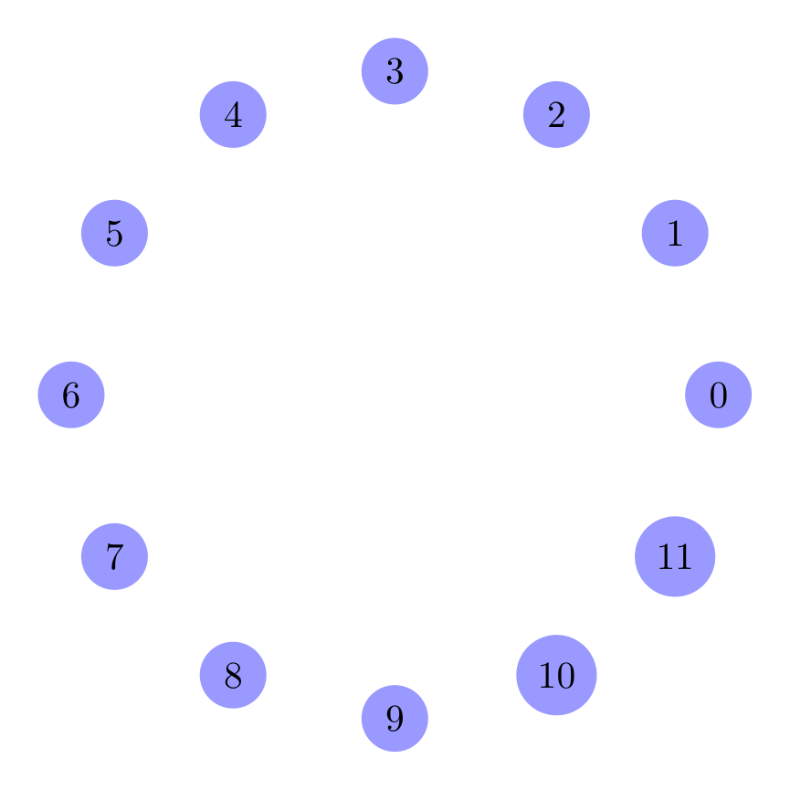
Show the TikZ code
% --------------------------------------------- %% Tikzfigure generated by tikzfigure v0.5.0 %% https://github.com/max-models/tikzfigure %% --------------------------------------------- %\begin{tikzpicture} \pgfmathsetmacro{\radius}{3} \node[shape=circle, fill=blue!40, minimum size=0.6cm] (node0) at ({{\radius*1.0000}}, {{\radius*0.0000}}) {0}; \node[shape=circle, fill=blue!40, minimum size=0.6cm] (node1) at ({{\radius*0.8661}}, {{\radius*0.4998}}) {1}; \node[shape=circle, fill=blue!40, minimum size=0.6cm] (node2) at ({{\radius*0.4998}}, {{\radius*0.8661}}) {2}; \node[shape=circle, fill=blue!40, minimum size=0.6cm] (node3) at ({{\radius*0.0000}}, {{\radius*1.0000}}) {3}; \node[shape=circle, fill=blue!40, minimum size=0.6cm] (node4) at ({{\radius*-0.4998}}, {{\radius*0.8661}}) {4}; \node[shape=circle, fill=blue!40, minimum size=0.6cm] (node5) at ({{\radius*-0.8661}}, {{\radius*0.4998}}) {5}; \node[shape=circle, fill=blue!40, minimum size=0.6cm] (node6) at ({{\radius*-1.0000}}, {{\radius*0.0000}}) {6}; \node[shape=circle, fill=blue!40, minimum size=0.6cm] (node7) at ({{\radius*-0.8661}}, {{\radius*-0.4998}}) {7}; \node[shape=circle, fill=blue!40, minimum size=0.6cm] (node8) at ({{\radius*-0.4998}}, {{\radius*-0.8661}}) {8}; \node[shape=circle, fill=blue!40, minimum size=0.6cm] (node9) at ({{\radius*-0.0000}}, {{\radius*-1.0000}}) {9}; \node[shape=circle, fill=blue!40, minimum size=0.6cm] (node10) at ({{\radius*0.4998}}, {{\radius*-0.8661}}) {10}; \node[shape=circle, fill=blue!40, minimum size=0.6cm] (node11) at ({{\radius*0.8661}}, {{\radius*-0.4998}}) {11};\end{tikzpicture}Show the standalone LaTeX document
\documentclass[border=10pt]{standalone}\PassOptionsToPackage{dvipsnames,svgnames,x11names}{xcolor}\usepackage{tikz}\usepackage{pgfplots}\pgfplotsset{compat=newest}\usepgfplotslibrary{groupplots}\usetikzlibrary{arrows.meta}\begin{document}% --------------------------------------------- %% Tikzfigure generated by tikzfigure v0.5.0     %% https://github.com/max-models/tikzfigure      %% --------------------------------------------- %\begin{tikzpicture}    \pgfmathsetmacro{\radius}{3}    \node[shape=circle, fill=blue!40, minimum size=0.6cm] (node0) at ({{\radius*1.0000}}, {{\radius*0.0000}}) {0};    \node[shape=circle, fill=blue!40, minimum size=0.6cm] (node1) at ({{\radius*0.8661}}, {{\radius*0.4998}}) {1};    \node[shape=circle, fill=blue!40, minimum size=0.6cm] (node2) at ({{\radius*0.4998}}, {{\radius*0.8661}}) {2};    \node[shape=circle, fill=blue!40, minimum size=0.6cm] (node3) at ({{\radius*0.0000}}, {{\radius*1.0000}}) {3};    \node[shape=circle, fill=blue!40, minimum size=0.6cm] (node4) at ({{\radius*-0.4998}}, {{\radius*0.8661}}) {4};    \node[shape=circle, fill=blue!40, minimum size=0.6cm] (node5) at ({{\radius*-0.8661}}, {{\radius*0.4998}}) {5};    \node[shape=circle, fill=blue!40, minimum size=0.6cm] (node6) at ({{\radius*-1.0000}}, {{\radius*0.0000}}) {6};    \node[shape=circle, fill=blue!40, minimum size=0.6cm] (node7) at ({{\radius*-0.8661}}, {{\radius*-0.4998}}) {7};    \node[shape=circle, fill=blue!40, minimum size=0.6cm] (node8) at ({{\radius*-0.4998}}, {{\radius*-0.8661}}) {8};    \node[shape=circle, fill=blue!40, minimum size=0.6cm] (node9) at ({{\radius*-0.0000}}, {{\radius*-1.0000}}) {9};    \node[shape=circle, fill=blue!40, minimum size=0.6cm] (node10) at ({{\radius*0.4998}}, {{\radius*-0.8661}}) {10};    \node[shape=circle, fill=blue!40, minimum size=0.6cm] (node11) at ({{\radius*0.8661}}, {{\radius*-0.4998}}) {11};\end{tikzpicture}
\end{document}