Images and legends
This tutorial covers what a pgfplots axis holds besides lines:
- A title, and labels with commas in them
- Ticks at chosen positions, with your own labels
- Filled polygons and colored points
- Images placed in data coordinates (
add_graphics) - Verbatim code in the axis coordinate system (
add_raw) - Legends that leave some plots out, placed anywhere
- Saving a figure together with its images
import io
import matplotlib
matplotlib.use("Agg")import matplotlib.pyplot as pltimport numpy as np
from tikzfigure import TikzFigure
Titles, labels and ticks
Section titled “Titles, labels and ticks”title= puts a title above the axis. Labels and titles that contain a comma or
= are braced for pgfplots automatically. set_ticks places ticks at the given
positions, optionally with your own labels.
fig = TikzFigure()ax = fig.axis2d(    title="Measurements, first week",    xlabel="day",    ylabel="temperature, $^\\circ$C",    xlim=(0, 6),    ylim=(10, 25),)ax.add_plot([0, 1, 2, 3, 4, 5, 6], [14, 15, 19, 22, 21, 18, 16], color="red", mark="*")ax.set_ticks("x", [0, 2, 4, 6], ["Mon", "Wed", "Fri", "Sun"])
fig.show()
/home/runner/work/tikzfigure/tikzfigure/.venv/lib/python3.12/site-packages/fitz/__init__.py:17: FutureWarning: The `fitz` API is deprecated and will be removed in future. Use `import pymupdf` instead. warnings.warn(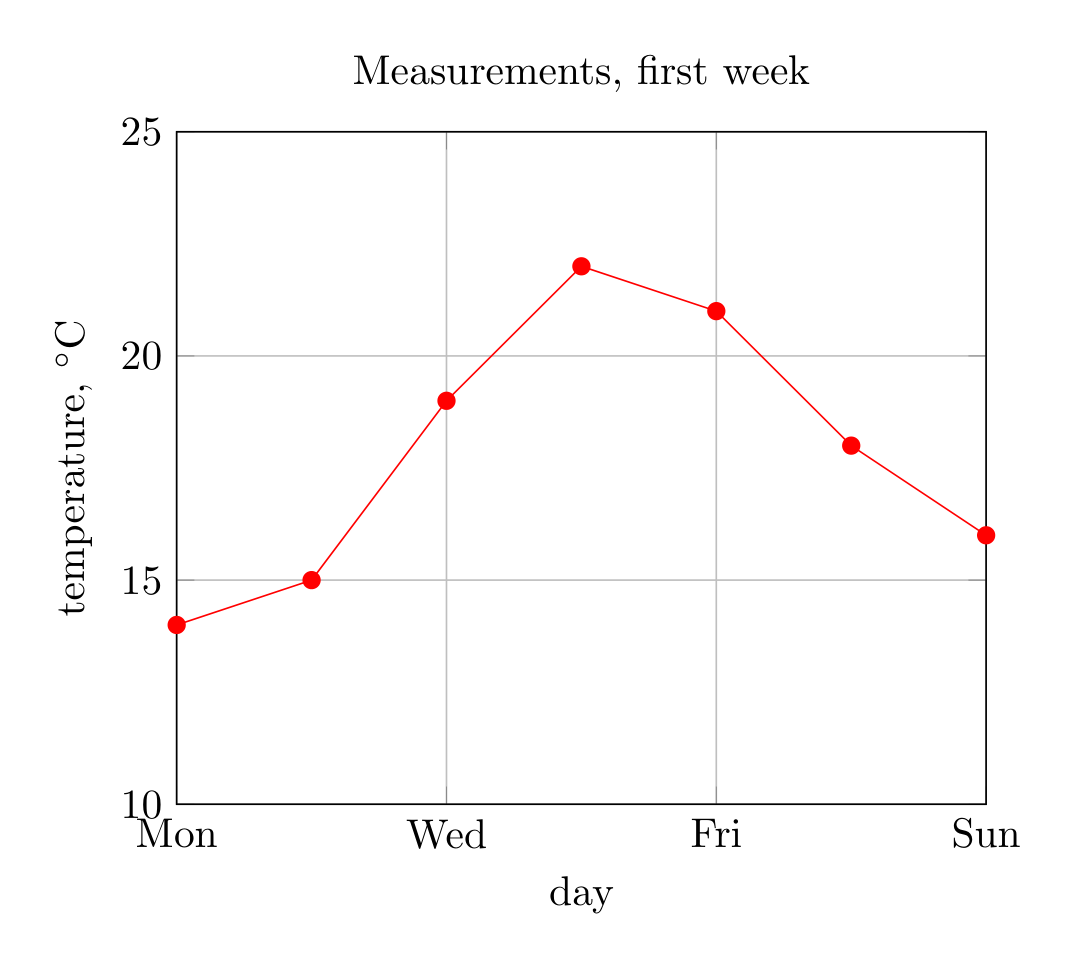
Show the TikZ code
% --------------------------------------------- %% Tikzfigure generated by tikzfigure v0.5.0 %% https://github.com/max-models/tikzfigure %% --------------------------------------------- %\begin{tikzpicture} \begin{axis}[title={Measurements, first week}, xlabel=day, ylabel={temperature, $^\circ$C}, xmin=0, xmax=6, ymin=10, ymax=25, xtick={0,2,4,6}, xticklabels={{Mon},{Wed},{Fri},{Sun}}, grid=major] \addplot[color=red, mark=*] coordinates {(0,14) (1,15) (2,19) (3,22) (4,21) (5,18) (6,16)}; \end{axis}\end{tikzpicture}Show the standalone LaTeX document
\documentclass[border=10pt]{standalone}\PassOptionsToPackage{dvipsnames,svgnames,x11names}{xcolor}\usepackage{tikz}\usepackage{pgfplots}\pgfplotsset{compat=newest}\usepgfplotslibrary{groupplots}\usetikzlibrary{arrows.meta}\usepackage{pgfplots}\begin{document}% --------------------------------------------- %% Tikzfigure generated by tikzfigure v0.5.0     %% https://github.com/max-models/tikzfigure      %% --------------------------------------------- %\begin{tikzpicture}    \begin{axis}[title={Measurements, first week}, xlabel=day, ylabel={temperature, $^\circ$C}, xmin=0, xmax=6, ymin=10, ymax=25, xtick={0,2,4,6}, xticklabels={{Mon},{Wed},{Fri},{Sun}}, grid=major]        \addplot[color=red, mark=*] coordinates {(0,14) (1,15) (2,19) (3,22) (4,21) (5,18) (6,16)};    \end{axis}\end{tikzpicture}
\end{document}
Filled polygons and colored points
Section titled “Filled polygons and colored points”cycle=True closes a plot’s path back to its first point, for a polygon.
meta= gives every point a value, written as (x,y) [value]; with the pgfplots
options scatter and point meta=explicit the points are colored by it
through the axis colormap.
fig = TikzFigure()ax = fig.axis2d(xlim=(0, 4), ylim=(0, 3), colorbar=True)ax.add_plot([0.5, 2.0, 1.2], [0.5, 0.8, 2.5], cycle=True, fill="blue", fill_opacity=0.2)
x = np.linspace(0.5, 3.5, 12)ax.add_plot(    x.tolist(),    (1.5 + np.sin(2 * x)).tolist(),    meta=x.tolist(),    options=["scatter", "only marks", "point meta=explicit"],)
fig.show()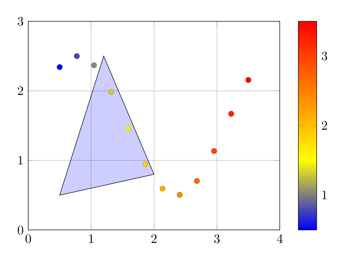
Show the TikZ code
% --------------------------------------------- %% Tikzfigure generated by tikzfigure v0.5.0 %% https://github.com/max-models/tikzfigure %% --------------------------------------------- %\begin{tikzpicture} \begin{axis}[xmin=0, xmax=4, ymin=0, ymax=3, grid=major, colorbar=true] \addplot[fill=blue, fill opacity=0.2] coordinates {(0.5,0.5) (2.0,0.8) (1.2,2.5)} -- cycle; \addplot[scatter, only marks, point meta=explicit] coordinates {(0.5,2.3414709848078967) [0.5] (0.7727272727272727,2.4996789142433977) [0.7727272727272727] (1.0454545454545454,2.36776314391168) [1.0454545454545454] (1.3181818181818181,1.984007857665163) [1.3181818181818181] (1.5909090909090908,1.4597853190024037) [1.5909090909090908] (1.8636363636363635,0.9472337597608833) [1.8636363636363635] (2.1363636363636362,0.5951042964940122) [2.1363636363636362] (2.409090909090909,0.5055908448925597) [2.409090909090909] (2.6818181818181817,0.7046717199810077) [2.6818181818181817] (2.954545454545454,1.1345702904724295) [2.954545454545454] (3.227272727272727,1.6705227326844927) [3.227272727272727] (3.5,2.156986598718789) [3.5]}; \end{axis}\end{tikzpicture}Show the standalone LaTeX document
\documentclass[border=10pt]{standalone}\PassOptionsToPackage{dvipsnames,svgnames,x11names}{xcolor}\usepackage{tikz}\usepackage{pgfplots}\pgfplotsset{compat=newest}\usepgfplotslibrary{groupplots}\usetikzlibrary{arrows.meta}\usepackage{pgfplots}\begin{document}% --------------------------------------------- %% Tikzfigure generated by tikzfigure v0.5.0     %% https://github.com/max-models/tikzfigure      %% --------------------------------------------- %\begin{tikzpicture}    \begin{axis}[xmin=0, xmax=4, ymin=0, ymax=3, grid=major, colorbar=true]        \addplot[fill=blue, fill opacity=0.2] coordinates {(0.5,0.5) (2.0,0.8) (1.2,2.5)} -- cycle;        \addplot[scatter, only marks, point meta=explicit] coordinates {(0.5,2.3414709848078967) [0.5] (0.7727272727272727,2.4996789142433977) [0.7727272727272727] (1.0454545454545454,2.36776314391168) [1.0454545454545454] (1.3181818181818181,1.984007857665163) [1.3181818181818181] (1.5909090909090908,1.4597853190024037) [1.5909090909090908] (1.8636363636363635,0.9472337597608833) [1.8636363636363635] (2.1363636363636362,0.5951042964940122) [2.1363636363636362] (2.409090909090909,0.5055908448925597) [2.409090909090909] (2.6818181818181817,0.7046717199810077) [2.6818181818181817] (2.954545454545454,1.1345702904724295) [2.954545454545454] (3.227272727272727,1.6705227326844927) [3.227272727272727] (3.5,2.156986598718789) [3.5]};    \end{axis}\end{tikzpicture}
\end{document}
precision= limits the digits of the written coordinates, which keeps long
data series readable: ax.add_plot(x, y, precision=4).
Images in data coordinates
Section titled “Images in data coordinates”Large colormap data would be slow and memory hungry as pgfplots coordinates.
add_graphics places an image instead, its edges at the given data
coordinates. Give an existing file as path=, or the image bytes as data=:
the figure then writes them next to the TikZ code when it compiles or saves it.
x, y = np.meshgrid(np.linspace(-2, 2, 200), np.linspace(-1, 1, 100))field = np.exp(-(x**2) - 4 * y**2) * np.cos(4 * x)png = io.BytesIO()plt.imsave(png, field, cmap="RdBu_r", origin="lower", format="png")
fig = TikzFigure()ax = fig.axis2d(xlabel="$x$", ylabel="$y$", xlim=(-2, 2), ylim=(-1, 1), grid=False)ax.add_graphics(-2, 2, -1, 1, data=png.getvalue(), filename="field.png")ax.add_plot([-2, 2], [0, 0], color="black", dashed=True)
fig.show()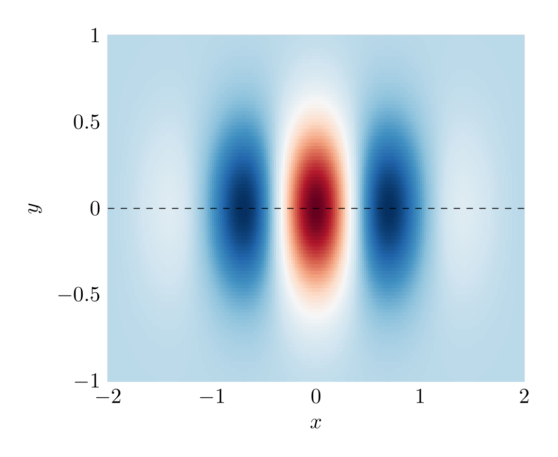
Show the TikZ code
% --------------------------------------------- %% Tikzfigure generated by tikzfigure v0.5.0 %% https://github.com/max-models/tikzfigure %% --------------------------------------------- %\begin{tikzpicture} \begin{axis}[xlabel=$x$, ylabel=$y$, xmin=-2, xmax=2, ymin=-1, ymax=1, grid=none] \addplot graphics[xmin=-2.0, xmax=2.0, ymin=-1.0, ymax=1.0] {field.png}; \addplot[color=black, dashed=true] coordinates {(-2,0) (2,0)}; \end{axis}\end{tikzpicture}Show the standalone LaTeX document
\documentclass[border=10pt]{standalone}\PassOptionsToPackage{dvipsnames,svgnames,x11names}{xcolor}\usepackage{tikz}\usepackage{pgfplots}\pgfplotsset{compat=newest}\usepgfplotslibrary{groupplots}\usetikzlibrary{arrows.meta}\usepackage{pgfplots}\begin{document}% --------------------------------------------- %% Tikzfigure generated by tikzfigure v0.5.0     %% https://github.com/max-models/tikzfigure      %% --------------------------------------------- %\begin{tikzpicture}    \begin{axis}[xlabel=$x$, ylabel=$y$, xmin=-2, xmax=2, ymin=-1, ymax=1, grid=none]        \addplot graphics[xmin=-2.0, xmax=2.0, ymin=-1.0, ymax=1.0] {field.png};        \addplot[color=black, dashed=true] coordinates {(-2,0) (2,0)};    \end{axis}\end{tikzpicture}
\end{document}
The plots, images and raw code of an axis are drawn in the order they were
added, so the dashed line is on top of the image. fig.files() lists the
images the figure needs:
list(fig.files())['field.png']Raw code in the axis coordinate system
Section titled “Raw code in the axis coordinate system”add_raw inserts verbatim code inside the axis, where axis cs: refers to data
coordinates and axis description cs: to the axis box, (0,0) at its lower
left and (1,1) at its upper right.
fig = TikzFigure()ax = fig.axis2d(xlim=(0, 10), ylim=(0, 1))ax.add_plot([0, 2, 4, 6, 8, 10], [0.1, 0.5, 0.9, 0.6, 0.3, 0.2], color="teal")ax.add_raw(r"\draw[->, thick] (axis cs:6,0.9) -- (axis cs:4.3,0.9);")ax.add_raw(r"\node[anchor=west] at (axis cs:6,0.9) {maximum};")ax.add_raw(r"\node[anchor=north east] at (axis description cs:0.98,0.98) {(a)};")
fig.show()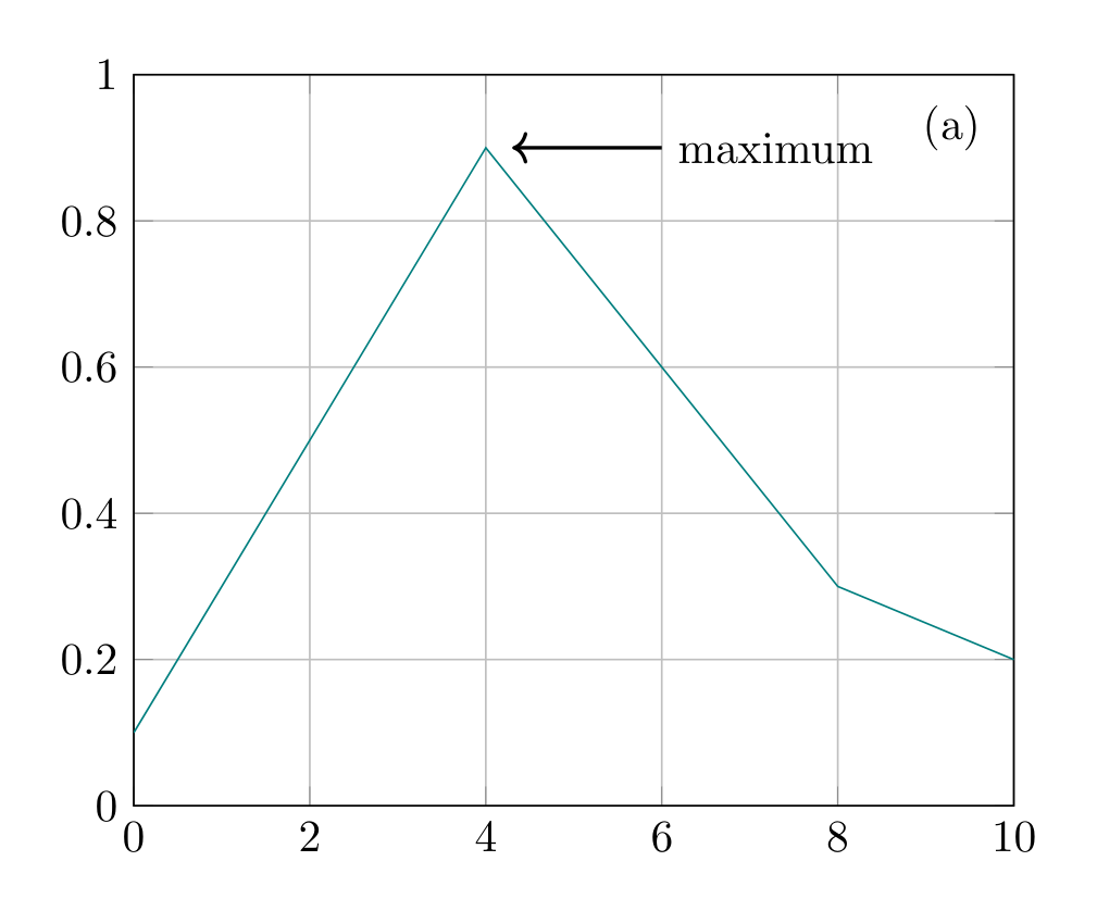
Show the TikZ code
% --------------------------------------------- %% Tikzfigure generated by tikzfigure v0.5.0 %% https://github.com/max-models/tikzfigure %% --------------------------------------------- %\begin{tikzpicture} \begin{axis}[xmin=0, xmax=10, ymin=0, ymax=1, grid=major] \addplot[color=teal] coordinates {(0,0.1) (2,0.5) (4,0.9) (6,0.6) (8,0.3) (10,0.2)}; \draw[->, thick] (axis cs:6,0.9) -- (axis cs:4.3,0.9); \node[anchor=west] at (axis cs:6,0.9) {maximum}; \node[anchor=north east] at (axis description cs:0.98,0.98) {(a)}; \end{axis}\end{tikzpicture}Show the standalone LaTeX document
\documentclass[border=10pt]{standalone}\PassOptionsToPackage{dvipsnames,svgnames,x11names}{xcolor}\usepackage{tikz}\usepackage{pgfplots}\pgfplotsset{compat=newest}\usepgfplotslibrary{groupplots}\usetikzlibrary{arrows.meta}\usepackage{pgfplots}\begin{document}% --------------------------------------------- %% Tikzfigure generated by tikzfigure v0.5.0     %% https://github.com/max-models/tikzfigure      %% --------------------------------------------- %\begin{tikzpicture}    \begin{axis}[xmin=0, xmax=10, ymin=0, ymax=1, grid=major]        \addplot[color=teal] coordinates {(0,0.1) (2,0.5) (4,0.9) (6,0.6) (8,0.3) (10,0.2)};        \draw[->, thick] (axis cs:6,0.9) -- (axis cs:4.3,0.9);        \node[anchor=west] at (axis cs:6,0.9) {maximum};        \node[anchor=north east] at (axis description cs:0.98,0.98) {(a)};    \end{axis}\end{tikzpicture}
\end{document}
Legends
Section titled “Legends”Plots with a label get a legend entry. If some plots have none, they are left
out of the legend (forget plot) instead of taking the next entry. at= places
the legend at a point of the axis box, anchor= says which point of the legend
goes there.
fig = TikzFigure()ax = fig.axis2d(xlabel="$t$", ylabel="signal", xlim=(0, 10), ylim=(-1.5, 1.5))t = np.linspace(0, 10, 60)ax.add_plot(    t.tolist(), np.sin(t).tolist(), label="measured, raw", color="blue", precision=4)ax.add_plot([0, 10], [0, 0], color="gray")  # a reference line, not in the legendax.add_plot(    t.tolist(), np.sin(t + 0.2).tolist(), label="model", color="red", precision=4)ax.set_legend(at=(0.02, 0.02), anchor="south west", columns=2, style="draw=none")
fig.show()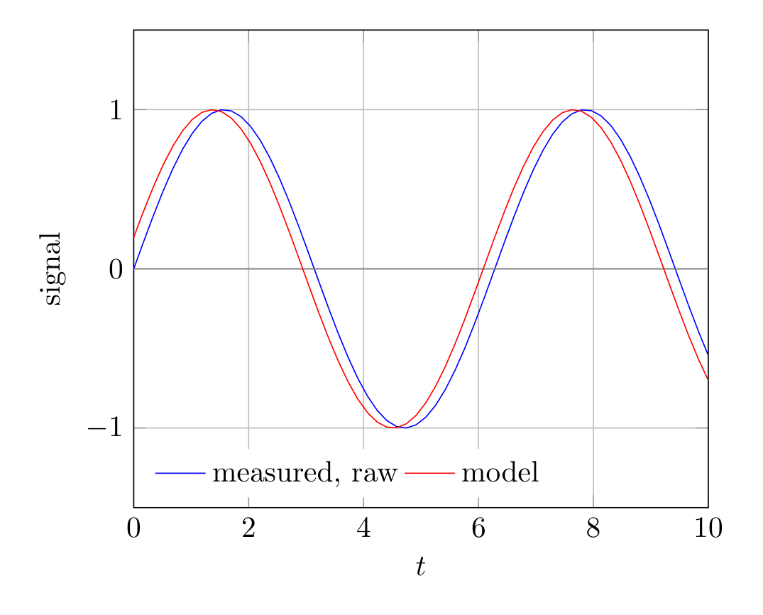
Show the TikZ code
% --------------------------------------------- %% Tikzfigure generated by tikzfigure v0.5.0 %% https://github.com/max-models/tikzfigure %% --------------------------------------------- %\begin{tikzpicture} \begin{axis}[xlabel=$t$, ylabel=signal, xmin=0, xmax=10, ymin=-1.5, ymax=1.5, grid=major, legend style={at={(0.02,0.02)}, anchor=south west, draw=none}, legend columns=2] \addplot[color=blue] coordinates {(0,0) (0.1695,0.1687) (0.339,0.3325) (0.5085,0.4868) (0.678,0.6272) (0.8475,0.7496) (1.017,0.8505) (1.186,0.927) (1.356,0.977) (1.525,0.999) (1.695,0.9923) (1.864,0.9572) (2.034,0.8947) (2.203,0.8065) (2.373,0.6952) (2.542,0.564) (2.712,0.4166) (2.881,0.2573) (3.051,0.09062) (3.22,-0.07866) (3.39,-0.2457) (3.559,-0.4057) (3.729,-0.554) (3.898,-0.6865) (4.068,-0.7993) (4.237,-0.8892) (4.407,-0.9537) (4.576,-0.9908) (4.746,-0.9994) (4.915,-0.9795) (5.085,-0.9315) (5.254,-0.8568) (5.424,-0.7575) (5.593,-0.6365) (5.763,-0.4973) (5.932,-0.3438) (6.102,-0.1805) (6.271,-0.012) (6.441,0.1568) (6.61,0.3212) (6.78,0.4763) (6.949,0.6178) (7.119,0.7416) (7.288,0.8441) (7.458,0.9225) (7.627,0.9744) (7.797,0.9984) (7.966,0.9937) (8.136,0.9606) (8.305,0.9) (8.475,0.8135) (8.644,0.7038) (8.814,0.5739) (8.983,0.4275) (9.153,0.2689) (9.322,0.1026) (9.492,-0.0667) (9.661,-0.234) (9.831,-0.3947) (10,-0.544)}; \addlegendentry{measured, raw} \addplot[color=gray, forget plot] coordinates {(0,0) (10,0)}; \addplot[color=red] coordinates {(0,0.1987) (0.1695,0.3611) (0.339,0.5133) (0.5085,0.6507) (0.678,0.7694) (0.8475,0.8662) (1.017,0.938) (1.186,0.9831) (1.356,0.9999) (1.525,0.9881) (1.695,0.9479) (1.864,0.8806) (2.034,0.7881) (2.203,0.673) (2.373,0.5385) (2.542,0.3887) (2.712,0.2277) (2.881,0.0602) (3.051,-0.109) (3.22,-0.2752) (3.39,-0.4334) (3.559,-0.5792) (3.729,-0.7084) (3.898,-0.8173) (4.068,-0.9028) (4.237,-0.9624) (4.407,-0.9944) (4.576,-0.998) (4.746,-0.9729) (4.915,-0.9199) (5.085,-0.8406) (5.254,-0.7372) (5.424,-0.6127) (5.593,-0.4706) (5.763,-0.315) (5.932,-0.1504) (6.102,0.01851) (6.271,0.1869) (6.441,0.3499) (6.61,0.5029) (6.78,0.6415) (6.949,0.7617) (7.119,0.8601) (7.288,0.9338) (7.458,0.9808) (7.627,0.9996) (7.797,0.9898) (7.966,0.9517) (8.136,0.8862) (8.305,0.7954) (8.475,0.6818) (8.644,0.5486) (8.814,0.3997) (8.983,0.2394) (9.153,0.07217) (9.322,-0.0971) (9.492,-0.2636) (9.661,-0.4225) (9.831,-0.5694) (10,-0.6999)}; \addlegendentry{model} \end{axis}\end{tikzpicture}Show the standalone LaTeX document
\documentclass[border=10pt]{standalone}\PassOptionsToPackage{dvipsnames,svgnames,x11names}{xcolor}\usepackage{tikz}\usepackage{pgfplots}\pgfplotsset{compat=newest}\usepgfplotslibrary{groupplots}\usetikzlibrary{arrows.meta}\usepackage{pgfplots}\begin{document}% --------------------------------------------- %% Tikzfigure generated by tikzfigure v0.5.0     %% https://github.com/max-models/tikzfigure      %% --------------------------------------------- %\begin{tikzpicture}    \begin{axis}[xlabel=$t$, ylabel=signal, xmin=0, xmax=10, ymin=-1.5, ymax=1.5, grid=major, legend style={at={(0.02,0.02)}, anchor=south west, draw=none}, legend columns=2]        \addplot[color=blue] coordinates {(0,0) (0.1695,0.1687) (0.339,0.3325) (0.5085,0.4868) (0.678,0.6272) (0.8475,0.7496) (1.017,0.8505) (1.186,0.927) (1.356,0.977) (1.525,0.999) (1.695,0.9923) (1.864,0.9572) (2.034,0.8947) (2.203,0.8065) (2.373,0.6952) (2.542,0.564) (2.712,0.4166) (2.881,0.2573) (3.051,0.09062) (3.22,-0.07866) (3.39,-0.2457) (3.559,-0.4057) (3.729,-0.554) (3.898,-0.6865) (4.068,-0.7993) (4.237,-0.8892) (4.407,-0.9537) (4.576,-0.9908) (4.746,-0.9994) (4.915,-0.9795) (5.085,-0.9315) (5.254,-0.8568) (5.424,-0.7575) (5.593,-0.6365) (5.763,-0.4973) (5.932,-0.3438) (6.102,-0.1805) (6.271,-0.012) (6.441,0.1568) (6.61,0.3212) (6.78,0.4763) (6.949,0.6178) (7.119,0.7416) (7.288,0.8441) (7.458,0.9225) (7.627,0.9744) (7.797,0.9984) (7.966,0.9937) (8.136,0.9606) (8.305,0.9) (8.475,0.8135) (8.644,0.7038) (8.814,0.5739) (8.983,0.4275) (9.153,0.2689) (9.322,0.1026) (9.492,-0.0667) (9.661,-0.234) (9.831,-0.3947) (10,-0.544)};        \addlegendentry{measured, raw}        \addplot[color=gray, forget plot] coordinates {(0,0) (10,0)};        \addplot[color=red] coordinates {(0,0.1987) (0.1695,0.3611) (0.339,0.5133) (0.5085,0.6507) (0.678,0.7694) (0.8475,0.8662) (1.017,0.938) (1.186,0.9831) (1.356,0.9999) (1.525,0.9881) (1.695,0.9479) (1.864,0.8806) (2.034,0.7881) (2.203,0.673) (2.373,0.5385) (2.542,0.3887) (2.712,0.2277) (2.881,0.0602) (3.051,-0.109) (3.22,-0.2752) (3.39,-0.4334) (3.559,-0.5792) (3.729,-0.7084) (3.898,-0.8173) (4.068,-0.9028) (4.237,-0.9624) (4.407,-0.9944) (4.576,-0.998) (4.746,-0.9729) (4.915,-0.9199) (5.085,-0.8406) (5.254,-0.7372) (5.424,-0.6127) (5.593,-0.4706) (5.763,-0.315) (5.932,-0.1504) (6.102,0.01851) (6.271,0.1869) (6.441,0.3499) (6.61,0.5029) (6.78,0.6415) (6.949,0.7617) (7.119,0.8601) (7.288,0.9338) (7.458,0.9808) (7.627,0.9996) (7.797,0.9898) (7.966,0.9517) (8.136,0.8862) (8.305,0.7954) (8.475,0.6818) (8.644,0.5486) (8.814,0.3997) (8.983,0.2394) (9.153,0.07217) (9.322,-0.0971) (9.492,-0.2636) (9.661,-0.4225) (9.831,-0.5694) (10,-0.6999)};        \addlegendentry{model}    \end{axis}\end{tikzpicture}
\end{document}
Saving with images
Section titled “Saving with images”savefig("figure.tikz") writes the tikzpicture, for \input into a document
that loads pgfplots; savefig("figure.tex") a standalone document. Both write
the images the figure refers to next to the file. .pdf and .png compile the
figure with them.