xarray data

Download notebook View on GitHubRun when the site was built.

maxplotlib understands labelled xarray data. Hand it a DataArray and it takes the coordinates for the axes, builds axis labels from the long_name and units attributes, and titles the plot with the coordinates you selected. Because the result is an ordinary Canvas, the same plot renders with every backend: Matplotlib, Plotly, plotext or TikZ.

There are two ways in:

Canvas methods such as canvas.plot(da), canvas.pcolormesh(da) and Canvas.facet(da, ...), which fit in with the rest of maxplotlib.
The .maxplot accessor, da.maxplot.line() and friends, which mirrors xarray’s own da.plot.line() API. Enable it with import maxplotlib.xarray.

xarray is optional: install it with pip install maxplotlibx[xarray]. maxplotlib never imports it for you.

import numpy as np
import xarray as xr

import maxplotlib.xarray  # noqa: F401  # registers da.maxplot and ds.maxplot
from maxplotlib import Canvas

A labelled line

A 1-D DataArray is plotted against its coordinate. The axis labels come from the attributes: long_name (falling back to the variable name) plus [units].

t = np.linspace(0, 10, 400)
energy = xr.DataArray(
    np.exp(-0.2 * t) * np.cos(3 * t) ** 2,
    dims="t",
    coords={"t": ("t", t, {"long_name": "Time", "units": "s"})},
    name="energy",
    attrs={"long_name": "Field energy", "units": "J"},
)

canvas = Canvas(width="12cm", ratio=0.5)
canvas.plot(energy, color="steelblue")
canvas.show()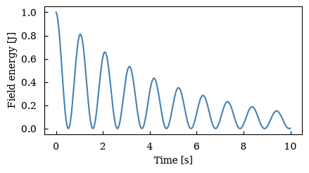

(<Figure size 472.441x236.22 with 1 Axes>,
 array([[<Axes: xlabel='Time [s]', ylabel='Field energy [J]'>]],
       dtype=object))

Labels you set yourself always win, whether you set them before or after plotting the array.

canvas = Canvas(width="12cm", ratio=0.5)
canvas.set_ylabel("$W$ [J]")
canvas.plot(energy, color="steelblue")
canvas.show()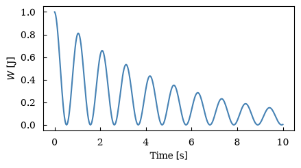

(<Figure size 472.441x236.22 with 1 Axes>,
 array([[<Axes: xlabel='Time [s]', ylabel='$W$ [J]'>]], dtype=object))

Choose the backend when rendering

da.maxplot.line() returns a Canvas; it doesn’t draw anything yet. Choose the backend when you show or save it, so the same object gives you an interactive Plotly figure, a terminal plot or TikZ code.

canvas = energy.maxplot.line(canvas_kwargs={"width": "12cm", "ratio": 0.5})
fig = canvas.show(backend="plotly")
fig

canvas.show(backend="plotext")

    ┌──────────────────────────────────────────────────────────────────────────┐
1.00┤▗                                                                         │
    │▝▖                                                                        │
    │ ▘                                                                        │
    │ ▘     ▗▖                                                                 │
0.75┤ ▝     ▞▐                                                                 │
    │ ▝     ▌▝                                                                 │
    │ ▝    ▗  ▌     ▞▖                                                         │
    │  ▖   ▗  ▖    ▐ ▚                                                         │
    │  ▖   ▗  ▗    ▗ ▝     ▗█                                                  │
0.50┤      ▖  ▗    ▘ ▝▖    ▞ ▌                                                 │
    │  ▝   ▖   ▖   ▌  ▖    ▌ ▚     ▞▚                                          │
    │  ▝  ▗    ▖  ▗   ▝   ▐  ▝▖   ▐▘▝▖     ▄▖                                  │
    │  ▗  ▗    ▖  ▗   ▝   ▗   ▖   ▞  ▚    ▞ ▜     ▗▄                           │
0.25┤   ▖ ▗    ▗  ▘   ▝▖  ▘   ▚   ▘  ▐    ▌  ▌   ▗▛▝▚     ▄▄                   │
    │   ▖ ▖    ▗  ▌    ▖ ▗▘   ▗  ▗▘   ▌  ▐   ▚   ▐  ▝▖   ▟▘▝▌    ▗▀▙     ▗▄    │
    │   ▘ ▘    ▝▖▗     ▚ ▐    ▝▖ ▞    ▚  ▛   ▝▖  ▌   ▙  ▗▘  ▐▖  ▗▘ ▝▌   ▗▛▝▚   │
    │   ▐▗▘     ▖▐     ▐ ▌     ▌▗▌    ▐▖▐     ▙ ▞    ▝▖ ▞    ▚ ▗▛   ▐▖ ▗▘   ▙  │
0.00┤   ▝▀      ▝▘      ▀▘     ▝▀      ▀▘     ▝▀▘     ▝▀      ▀▀     ▝▀▘     ▀▘│
    └┬───────────┬───────────┬────────────┬───────────┬───────────┬───────────┬┘
     0.0        1.7         3.3          5.0         6.7         8.3       10.0
Field energy [J]                     Time [s]

<maxplotlib.backends.plotext.figure.PlotextFigure at 0x7f720d93dac0>

Titles from selections

After sel or isel, the selected values stay on the array as single-value coordinates. maxplotlib turns them into the title, with units, unless you set one.

x = np.linspace(0, 2 * np.pi, 80)
y = np.linspace(-1, 1, 50)
ts = np.linspace(0, 1.5, 6)
wave = xr.DataArray(
    np.sin(x[None, None, :] - 2 * ts[:, None, None])
    * np.exp(-3 * y[None, :, None] ** 2),
    dims=("t", "y", "x"),
    coords={
        "t": ("t", ts, {"units": "s"}),
        "y": ("y", y, {"long_name": "Height", "units": "m"}),
        "x": ("x", x, {"units": "m"}),
    },
    name="phi",
    attrs={"long_name": "Potential", "units": "V"},
)

wave.sel(t=0.6).isel(y=25).maxplot.line().show()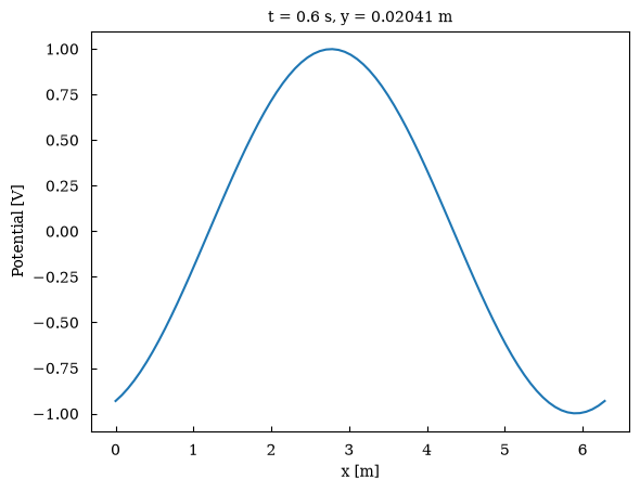

(<Figure size 640x480 with 1 Axes>,
 array([[<Axes: title={'center': 't = 0.6 s, y = 0.02041 m'}, xlabel='x [m]', ylabel='Potential [V]'>]],
       dtype=object))

Time series and categories

Datetime and text coordinates work as they are.

days = np.arange("2026-01-01", "2026-03-01", dtype="datetime64[D]")
temperature = xr.DataArray(
    5
    + 3 * np.sin(np.arange(days.size) / 9)
    + np.random.default_rng(0).normal(0, 0.6, days.size),
    dims="time",
    coords={"time": days},
    name="temperature",
    attrs={"units": "°C"},
)
canvas = temperature.maxplot.line(canvas_kwargs={"width": "12cm", "ratio": 0.45})
canvas.autofmt_xdate()
canvas.show()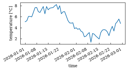

(<Figure size 472.441x212.598 with 1 Axes>,
 array([[<Axes: xlabel='time', ylabel='temperature [°C]'>]], dtype=object))

yields = xr.DataArray(
    [4.2, 3.1, 5.6, 2.4],
    dims="crop",
    coords={"crop": ["wheat", "barley", "maize", "oats"]},
    name="yield",
    attrs={"units": "t/ha"},
)
yields.maxplot.scatter(s=60).show()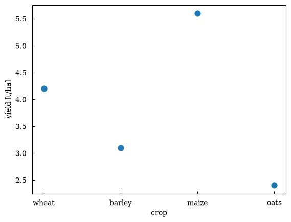

(<Figure size 640x480 with 1 Axes>,
 array([[<Axes: xlabel='crop', ylabel='yield [t/ha]'>]], dtype=object))

One line per value: `hue=`

A 2-D array draws as one line per value of the hue dimension. The lines are labelled dim = value, coloured C0, C1, … and the legend is switched on. Pass add_legend=False to hide it.

density = xr.DataArray(
    np.stack([np.exp(-t / 3), 0.8 * np.exp(-t / 5), 0.5 * np.exp(-t)]),
    dims=("species", "t"),
    coords={"species": ["ions", "electrons", "fast"], "t": energy.t},
    name="density",
    attrs={"units": "m^-3"},
)
density.maxplot.line(hue="species").show()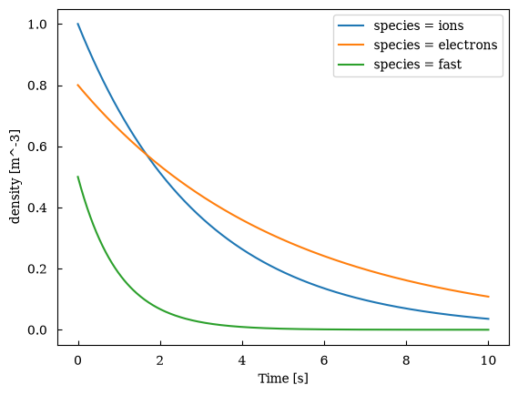

(<Figure size 640x480 with 1 Axes>,
 array([[<Axes: xlabel='Time [s]', ylabel='density [m^-3]'>]], dtype=object))

Choosing the coordinate for each axis

With the accessor, x= and y= name a dimension or coordinate, exactly as in xarray. On Canvas methods, where x and y are already the positional data arguments, the same options are called xcoord= and ycoord=.

x= can pick a non-dimension coordinate, and y= puts the coordinate on the y-axis for a vertical profile:

z = np.linspace(0, 12, 40)
temperature_profile = xr.DataArray(
    288 - 6.5 * np.minimum(z, 11) + 0.4 * np.sin(z),
    dims="level",
    coords={
        "z": ("level", z, {"long_name": "Altitude", "units": "km"}),
        "p": (
            "level",
            1013 * np.exp(-z / 8),
            {"long_name": "Pressure", "units": "hPa"},
        ),
    },
    name="T",
    attrs={"long_name": "Temperature", "units": "K"},
)

canvas, (left, right) = Canvas.subplots(ncols=2, width="14cm", ratio=0.45, wspace=0.35)
left.plot(temperature_profile, xcoord="p")
right.plot(temperature_profile, ycoord="z")
canvas.show()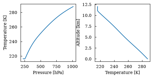

(<Figure size 551.181x248.031 with 2 Axes>,
 array([[<Axes: xlabel='Pressure [hPa]', ylabel='Temperature [K]'>,
         <Axes: xlabel='Temperature [K]', ylabel='Altitude [km]'>]],
       dtype=object))

2-D fields

pcolormesh, imshow, contourf and contour take a 2-D array. Like xarray, the first dimension goes on the y-axis. A labelled colorbar is added, except for contour; add_colorbar= changes that. Other keyword arguments go to the backend as usual, such as aspect="auto" to stretch the image to its axes.

field = wave.sel(t=0)
canvas, axes = Canvas.subplots(
    nrows=2, ncols=2, width="16cm", ratio=0.75, wspace=0.7, hspace=0.5
)
axes[0][0].pcolormesh(field)
axes[0][1].imshow(field, aspect="auto")
axes[1][0].contourf(field)
axes[1][1].contour(field, add_colorbar=True)
canvas.show()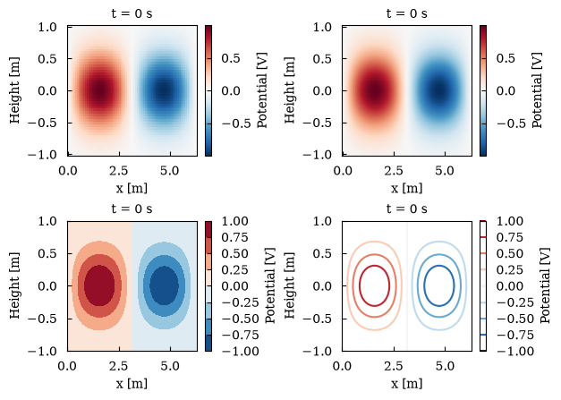

(<Figure size 629.921x472.441 with 8 Axes>,
 array([[<Axes: title={'center': 't = 0 s'}, xlabel='x [m]', ylabel='Height [m]'>,
         <Axes: title={'center': 't = 0 s'}, xlabel='x [m]', ylabel='Height [m]'>],
        [<Axes: title={'center': 't = 0 s'}, xlabel='x [m]', ylabel='Height [m]'>,
         <Axes: title={'center': 't = 0 s'}, xlabel='x [m]', ylabel='Height [m]'>]],
       dtype=object))

Swap the axes by naming the coordinates. Plots also combine: here are contour lines drawn over a mesh.

canvas = Canvas(width="10cm", ratio=0.8)
canvas.pcolormesh(field, xcoord="y", ycoord="x", cmap="magma", center=False)
canvas.contour(field, xcoord="y", ycoord="x", colors="white", levels=6)
canvas.show()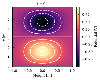

(<Figure size 393.701x314.961 with 2 Axes>,
 array([[<Axes: title={'center': 't = 0 s'}, xlabel='Height [m]', ylabel='x [m]'>]],
       dtype=object))

Colour defaults

Data with both signs gets a diverging colour map (RdBu_r) centred on zero, as in xarray. center= moves the centre and center=False turns this off. robust=True takes the colour limits from the 2nd and 98th percentiles, so a few outliers don’t wash out the plot.

noisy = field.copy()
noisy[10, 10] = 25  # a single outlier

canvas, (left, right) = Canvas.subplots(ncols=2, width="16cm", ratio=0.4, wspace=0.7)
left.pcolormesh(noisy)
left.set_title("default: the outlier sets the scale")
right.pcolormesh(noisy, robust=True)
right.set_title("robust=True")
canvas.show()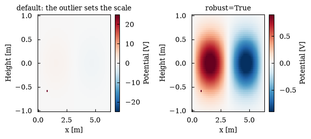

(<Figure size 629.921x251.969 with 4 Axes>,
 array([[<Axes: title={'center': 'default: the outlier sets the scale'}, xlabel='x [m]', ylabel='Height [m]'>,
         <Axes: title={'center': 'robust=True'}, xlabel='x [m]', ylabel='Height [m]'>]],
       dtype=object))

canvas = Canvas(width="8cm", ratio=0.8)
canvas.pcolormesh(field, center=False)
canvas.set_title("center=False: a sequential colour map")
canvas.show()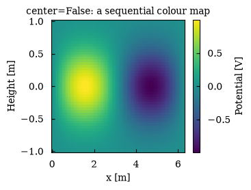

(<Figure size 314.961x251.969 with 2 Axes>,
 array([[<Axes: title={'center': 'center=False: a sequential colour map'}, xlabel='x [m]', ylabel='Height [m]'>]],
       dtype=object))

Curvilinear grids

Simulation output often lives on logical dimensions with 2-D physical coordinates, for example R(e1, e2) and Z(e1, e2). Name both coordinates to draw the field where it really is. This needs the Matplotlib backend; Plotly’s heatmaps and contours only support rectilinear grids.

e1 = np.linspace(0.2, 1, 30)[:, None]
e2 = np.linspace(0, 2 * np.pi, 90)[None, :]
R = 3 + e1 * np.cos(e2)
Z = 1.6 * e1 * np.sin(e2)
pressure = xr.DataArray(
    (1 - e1**2) * (1 + 0.15 * np.cos(3 * e2)),
    dims=("e1", "e2"),
    coords={
        "R": (("e1", "e2"), R, {"units": "m"}),
        "Z": (("e1", "e2"), Z, {"units": "m"}),
    },
    name="p",
    attrs={"long_name": "Pressure", "units": "kPa"},
)

canvas = pressure.maxplot.pcolormesh(
    x="R", y="Z", canvas_kwargs={"width": "8cm", "ratio": 1.1}
)
canvas.set_aspect("equal")
canvas.show()

/home/runner/work/maxplotlib/maxplotlib/src/maxplotlib/subfigure/line_plot.py:1635: UserWarning: The input coordinates to pcolormesh are interpreted as cell centers, but are not monotonically increasing or decreasing. This may lead to incorrectly calculated cell edges, in which case, please supply explicit cell edges to pcolormesh.
  im = ax.pcolormesh(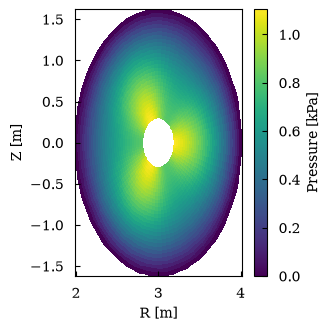

(<Figure size 314.961x346.457 with 2 Axes>,
 array([[<Axes: xlabel='R [m]', ylabel='Z [m]'>]], dtype=object))

col=, row= and col_wrap= lay the data out over a grid, one subplot per value. Colour-mapped plots share one colour scale and one colorbar. Axis and tick labels appear on the outer subplots only, and each subplot is titled with its value.

wave.maxplot.pcolormesh(
    col="t", col_wrap=3, canvas_kwargs={"width": "16cm", "ratio": 0.6}
).show()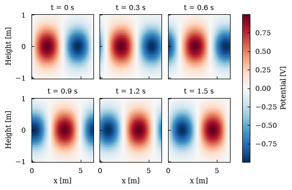

(<Figure size 629.921x377.953 with 7 Axes>,
 array([[<Axes: title={'center': 't = 0 s'}, ylabel='Height [m]'>,
         <Axes: title={'center': 't = 0.3 s'}>,
         <Axes: title={'center': 't = 0.6 s'}>],
        [<Axes: title={'center': 't = 0.9 s'}, xlabel='x [m]', ylabel='Height [m]'>,
         <Axes: title={'center': 't = 1.2 s'}, xlabel='x [m]'>,
         <Axes: title={'center': 't = 1.5 s'}, xlabel='x [m]'>]],
       dtype=object))

Line facets share their value range too, which makes panels easy to compare. sharey=False gives each panel its own scale. Coordinates that all panels share (here the selected height) move into the figure title.

wave.sel(y=0, method="nearest").maxplot.line(
    col="t", col_wrap=3, canvas_kwargs={"width": "16cm", "ratio": 0.5}
).show()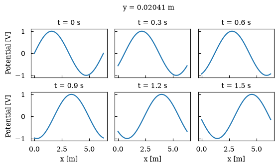

(<Figure size 629.921x314.961 with 6 Axes>,
 array([[<Axes: title={'center': 't = 0 s'}, ylabel='Potential [V]'>,
         <Axes: title={'center': 't = 0.3 s'}>,
         <Axes: title={'center': 't = 0.6 s'}>],
        [<Axes: title={'center': 't = 0.9 s'}, xlabel='x [m]', ylabel='Potential [V]'>,
         <Axes: title={'center': 't = 1.2 s'}, xlabel='x [m]'>,
         <Axes: title={'center': 't = 1.5 s'}, xlabel='x [m]'>]],
       dtype=object))

The accessor methods are shortcuts for Canvas.facet, which you can also call directly. Like Canvas.subplots, it returns the canvas and a grid of subplots, which you can keep editing. In Plotly, a label shared across subplots gets a single legend entry that toggles all of them.

runs = xr.concat(
    [density, 1.5 * density],
    dim=xr.DataArray(["baseline", "heated"], dims="run", name="run"),
)
canvas, axes = Canvas.facet(
    runs.isel(t=slice(0, None, 4)),
    col="run",
    kind="plot",
    hue="species",
    canvas_kwargs={"width": "15cm", "ratio": 0.4},
)
axes[0][0].set_yscale("log")
axes[0][1].set_yscale("log")
fig = canvas.show(backend="plotly")
fig

Datasets

ds.maxplot.line() and ds.maxplot.scatter() plot one variable against another. hue= may be a dimension, for one series per value, or, for scatter, another variable that colours the points.

rng = np.random.default_rng(1)
n = rng.uniform(1, 5, (3, 60))
plasma = xr.Dataset(
    {
        "n": (("species", "sample"), n, {"long_name": "Density", "units": "1e19 m^-3"}),
        "T": (
            ("species", "sample"),
            2 * n + rng.normal(0, 0.5, n.shape),
            {"long_name": "Temperature", "units": "keV"},
        ),
        "v": (
            ("species", "sample"),
            rng.normal(0, 1, n.shape),
            {"long_name": "Flow", "units": "km/s"},
        ),
    },
    coords={"species": ["D", "T", "e"]},
)

plasma.maxplot.scatter(x="n", y="T", hue="species").show()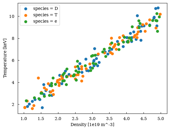

(<Figure size 640x480 with 1 Axes>,
 array([[<Axes: xlabel='Density [1e19 m^-3]', ylabel='Temperature [keV]'>]],
       dtype=object))

plasma.maxplot.scatter(x="n", y="T", hue="v").show()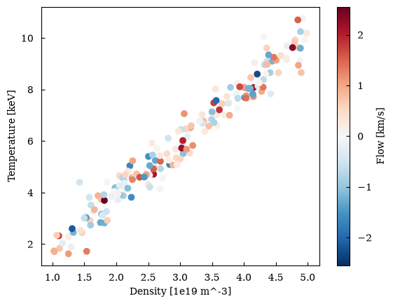

(<Figure size 640x480 with 2 Axes>,
 array([[<Axes: xlabel='Density [1e19 m^-3]', ylabel='Temperature [keV]'>]],
       dtype=object))

Units with pint

If the data is a pint Quantity, as with pint-xarray, maxplotlib reads the units from it and plots the plain magnitudes.

import pint

ureg = pint.UnitRegistry()
speed = xr.DataArray(
    ureg.Quantity(3 * np.sqrt(t), "m/s"),
    dims="t",
    coords={"t": energy.t},
    name="speed",
)
speed.maxplot.line().show()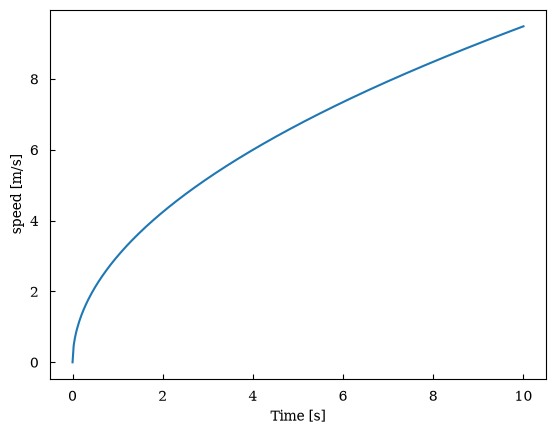

(<Figure size 640x480 with 1 Axes>,
 array([[<Axes: xlabel='Time [s]', ylabel='speed [m/s]'>]], dtype=object))

Part of the max-models projects Source on GitHub