Multiple subplots

Download notebookView on GitHubRun when the site was built.

This notebook shows all the ways to build multi-panel figures with maxplotlib:

• Canvas.subplots(ncols=...) / Canvas.subplots(nrows=..., ncols=...)
• squeeze=False for a consistent 2-D axes list
• Manual layout with canvas.add_subplot(row=..., col=...)
• Accessing subplots: canvas.subplot(), canvas[row, col], canvas.iter_subplots()
• Figure-level title with canvas.suptitle()
• Canvas-level plot routing to a specific subplot

import numpy as np
from tikzfigure import TikzFigure

from maxplotlib import Canvas

%matplotlib inline
%load_ext autoreload
%autoreload 2

x = np.linspace(0, 2 * np.pi, 200)

Backend selection

All examples in this tutorial use the same Canvas API; you can switch rendering backends at any time:

• BACKEND = "matplotlib" for static Matplotlib output
• BACKEND = "plotly" for interactive Plotly output (Jupyter-friendly)

Most cells end with canvas.show(backend=BACKEND) so you can re-run the whole notebook with a different backend.

# Change to "plotly" for interactive output
BACKEND = "matplotlib"

fig = TikzFigure()

x = np.linspace(0, 360, 200)
y1 = np.sin(np.radians(x))
y2 = np.cos(np.radians(x))

# First subfigure: sine wave
ax1 = fig.subfigure_axis(
    xlabel="x",
    ylabel="y",
    xlim=(0, 360),
    ylim=(-1.5, 1.5),
    grid=True,
    title="Sine Function",
    width=0.45,
)
ax1.add_plot(x=x, y=y1, label="sin(x)", color="red", line_width="1.5pt")
ax1.set_legend(position="north east")

# Second subfigure: cosine wave
ax2 = fig.subfigure_axis(
    xlabel="x",
    ylabel="y",
    xlim=(0, 360),
    ylim=(-1.5, 1.5),
    grid=True,
    title="Cosine Function",
    width=0.45,
)
ax2.add_plot(x=x, y=y2, label="cos(x)", color="blue", line_width="1.5pt")
ax2.set_legend(position="north east")

fig.show()

2026-10-30 07:52:23.669151421 [W:onnxruntime:Default, device_discovery.cc:95 GetPciBusId] Skipping pci_bus_id for PCI path at "/sys/devices/LNXSYSTM:00/LNXSYBUS:00/ACPI0004:00/MSFT1000:00/5620e0c7-8062-4dce-aeb7-520c7ef76171" because filename "5620e0c7-8062-4dce-aeb7-520c7ef76171" did not match expected pattern of [0-9a-f]+:[0-9a-f]+:[0-9a-f]+[.][0-9a-f]+
/home/runner/work/maxplotlib/maxplotlib/.venv/lib/python3.12/site-packages/fitz/__init__.py:17: FutureWarning: The `fitz` API is deprecated and will be removed in future. Use `import pymupdf` instead.
  warnings.warn(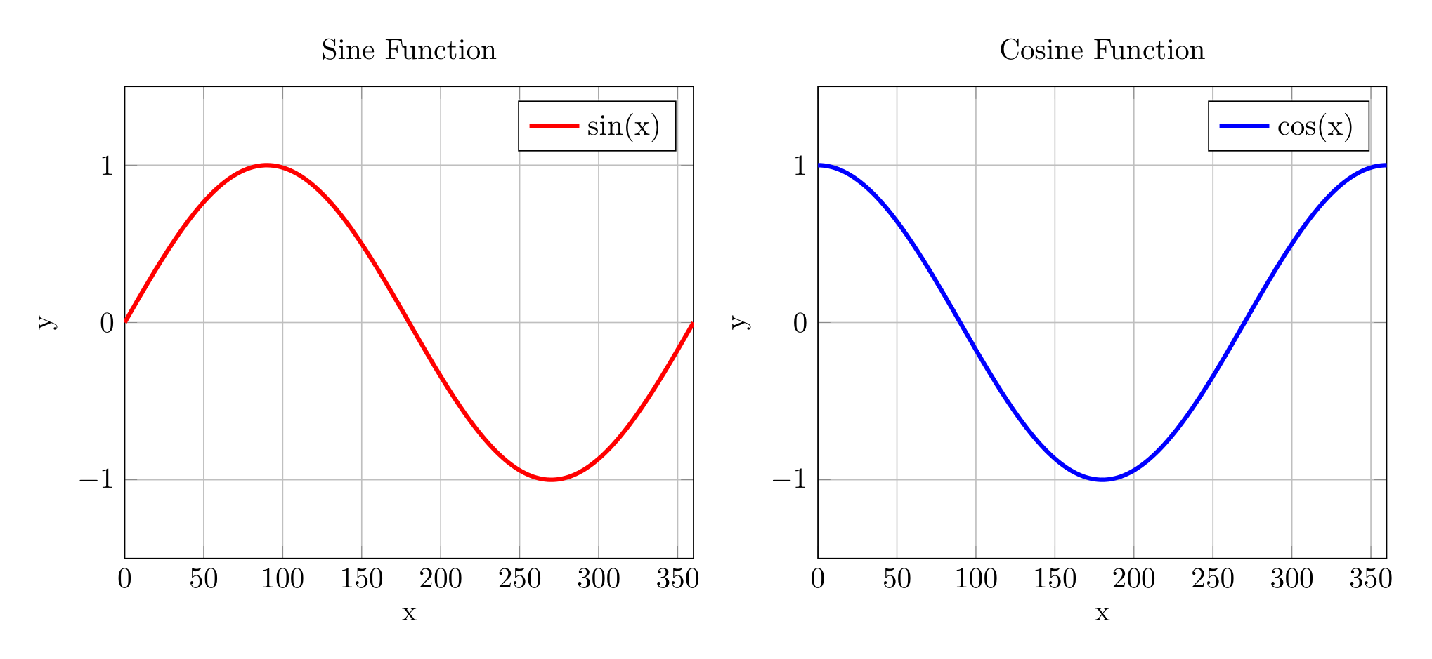

1 1×2 layout — side-by-side subplots

canvas, (ax1, ax2) = Canvas.subplots(ncols=2, width=1000, ratio=0.3)

x = np.linspace(0, 2 * np.pi, 200)

ax1.plot(x, np.sin(x), color="royalblue", linewidth=1.5)
ax1.set_title("sin(x)")
ax1.set_xlabel("x")
ax1.set_ylabel("amplitude")

ax2.plot(x, np.cos(x), color="tomato", linewidth=1.5)
ax2.set_title("cos(x)")
ax2.set_xlabel("x")

canvas.suptitle("1 × 2 Layout")
canvas.show(backend="tikzfigure")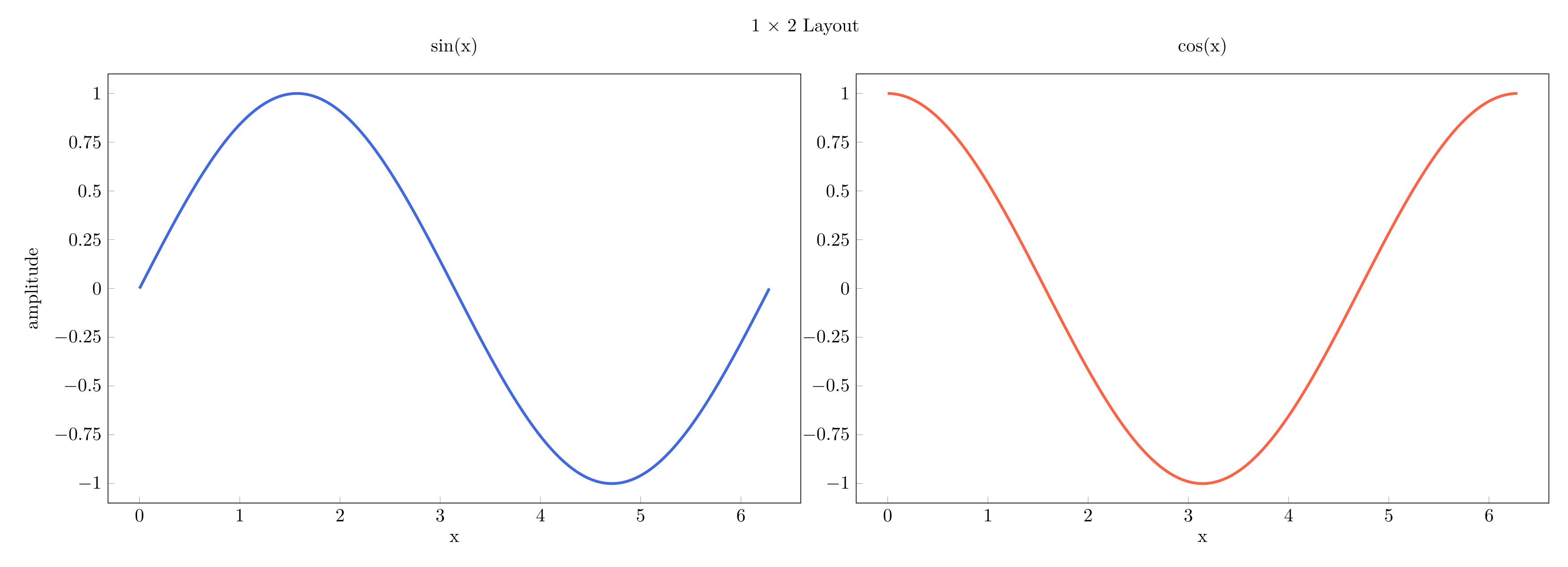

2 2×2 layout — grid of subplots

Canvas.subplots(nrows=2, ncols=2) returns a 2-D list of subplot axes indexed as axes[row][col].

canvas, axes = Canvas.subplots(nrows=2, ncols=2)

axes[0][0].plot(x, np.sin(x), color="royalblue")
axes[0][0].set_title("sin(x)")
axes[0][1].plot(x, np.cos(x), color="tomato")
axes[0][1].set_title("cos(x)")
axes[1][0].plot(x, np.sin(2 * x), color="seagreen")
axes[1][0].set_title("sin(2x)")
axes[1][1].plot(x, np.cos(2 * x), color="darkorange")
axes[1][1].set_title("cos(2x)")

canvas.suptitle("2 × 2 Layout")
canvas.show(backend=BACKEND)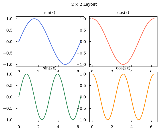

(<Figure size 640x480 with 4 Axes>,
 array([[<Axes: title={'center': 'sin(x)'}>,
         <Axes: title={'center': 'cos(x)'}>],
        [<Axes: title={'center': 'sin(2x)'}>,
         <Axes: title={'center': 'cos(2x)'}>]], dtype=object))

3 squeeze=False — always get a 2-D list

By default a 1×N or N×1 grid returns a flat list. Pass squeeze=False to always get a 2-D nested list — useful when your layout code must be generic.

canvas, axes = Canvas.subplots(nrows=1, ncols=3, squeeze=False)

# axes is always [[ax0, ax1, ax2]] — index as axes[row][col]
data = [np.sin(x), np.cos(x), np.tan(np.clip(x, 0, np.pi - 0.1))]
titles = ["sin", "cos", "tan (clipped)"]

for col, (d, t) in enumerate(zip(data, titles)):
    axes[0][col].plot(x, d, color="steelblue")
    axes[0][col].set_title(t)

canvas.show(backend=BACKEND)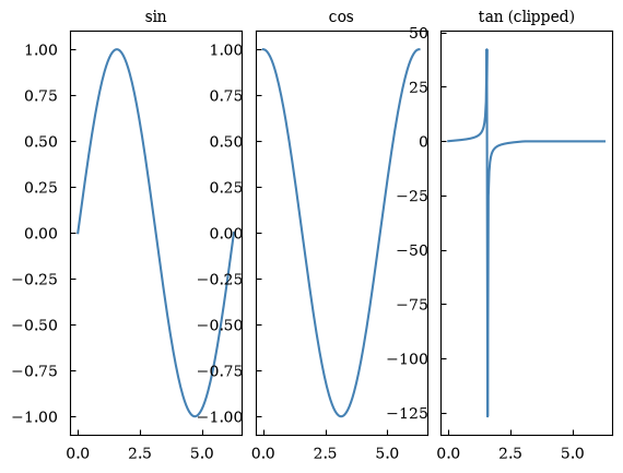

(<Figure size 640x480 with 3 Axes>,
 array([[<Axes: title={'center': 'sin'}>, <Axes: title={'center': 'cos'}>,
         <Axes: title={'center': 'tan (clipped)'}>]], dtype=object))

4 Manual layout — canvas.add_subplot(row, col)

You can build the layout yourself by calling add_subplot explicitly. This lets you configure each panel’s title, labels, grid, and legend in one shot.

canvas = Canvas(nrows=2, ncols=2)

ax00 = canvas.add_subplot(
    row=0, col=0, title="Top-left", xlabel="x", ylabel="y", grid=True
)
ax01 = canvas.add_subplot(row=0, col=1, title="Top-right", xlabel="x", grid=True)
ax10 = canvas.add_subplot(row=1, col=0, title="Bottom-left", xlabel="x", ylabel="y")
ax11 = canvas.add_subplot(row=1, col=1, title="Bottom-right", xlabel="x", legend=True)

ax00.plot(x, np.sin(x), color="royalblue")
ax01.plot(x, np.cos(x), color="tomato")
ax10.plot(x, np.sin(2 * x), color="seagreen")
ax11.plot(x, np.sin(x), label="sin", color="royalblue")
ax11.plot(x, np.cos(x), label="cos", color="tomato")

canvas.suptitle("Manual Layout")
canvas.show(backend=BACKEND)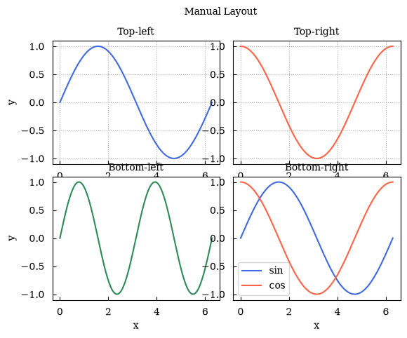

(<Figure size 640x480 with 4 Axes>,
 array([[<Axes: title={'center': 'Top-left'}, xlabel='x', ylabel='y'>,
         <Axes: title={'center': 'Top-right'}, xlabel='x'>],
        [<Axes: title={'center': 'Bottom-left'}, xlabel='x', ylabel='y'>,
         <Axes: title={'center': 'Bottom-right'}, xlabel='x'>]],
       dtype=object))

5 Accessing subplots after creation

Three equivalent ways to retrieve a subplot object:

canvas, axes = Canvas.subplots(nrows=2, ncols=2)

# Method A: use the object returned by subplots()
axes[0][0].set_title("Method A")

# Method B: canvas.subplot(row, col)
sp_b = canvas.subplot(row=0, col=1)
sp_b.set_title("Method B")

# Method C: canvas[row, col] indexing
canvas[1, 0].set_title("Method C")
canvas[1, 1].set_title("Method D (index)")

canvas.show(backend=BACKEND)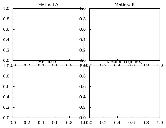

(<Figure size 640x480 with 4 Axes>,
 array([[<Axes: title={'center': 'Method A'}>,
         <Axes: title={'center': 'Method B'}>],
        [<Axes: title={'center': 'Method C'}>,
         <Axes: title={'center': 'Method D (index)'}>]], dtype=object))

6 canvas.iter_subplots() — loop over all panels

canvas, axes = Canvas.subplots(nrows=2, ncols=2)

# Plot something in every panel first
for row in range(2):
    for col in range(2):
        axes[row][col].plot(x, np.sin((row + 1) * (col + 1) * x))

# Then enable grid on every panel uniformly
for row, col, sp in canvas.iter_subplots():
    sp.set_grid(True)
    sp.set_xlabel("x")

canvas.show(backend=BACKEND)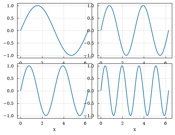

(<Figure size 640x480 with 4 Axes>,
 array([[<Axes: xlabel='x'>, <Axes: xlabel='x'>],
        [<Axes: xlabel='x'>, <Axes: xlabel='x'>]], dtype=object))

7 Canvas-level plot routing

Pass row= and col= to canvas-level methods to target a specific subplot.

canvas = Canvas(nrows=1, ncols=2)
canvas.add_subplot(row=0, col=0, title="Left", xlabel="x", ylabel="sin")
canvas.add_subplot(row=0, col=1, title="Right", xlabel="x", ylabel="cos")

canvas.plot(x, np.sin(x), row=0, col=0, color="royalblue", label="sin")
canvas.plot(x, np.cos(x), row=0, col=1, color="tomato", label="cos")

canvas.set_legend(True, row=0, col=0)
canvas.set_legend(True, row=0, col=1)
canvas.suptitle("Canvas-level routing")
canvas.show(backend=BACKEND)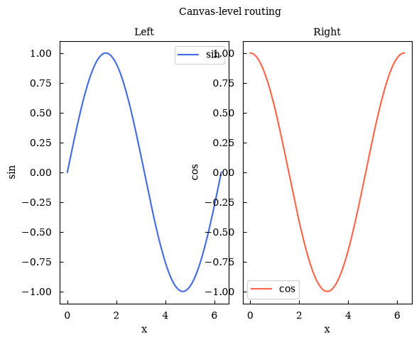

(<Figure size 640x480 with 2 Axes>,
 array([[<Axes: title={'center': 'Left'}, xlabel='x', ylabel='sin'>,
         <Axes: title={'center': 'Right'}, xlabel='x', ylabel='cos'>]],
       dtype=object))

Summary

Task	Code
1×2 grid	canvas, (ax1, ax2) = Canvas.subplots(ncols=2)
2×2 grid	canvas, axes = Canvas.subplots(nrows=2, ncols=2) — index axes[r][c]
Always 2-D	Canvas.subplots(..., squeeze=False)
Manual panel	canvas.add_subplot(row=r, col=c, ...)
Get subplot	canvas.subplot(r, c) or canvas[r, c]
Loop panels	for row, col, sp in canvas.iter_subplots()
Figure title	canvas.suptitle('...')
Route plot	canvas.plot(x, y, row=r, col=c)

Next: Tutorial 03 covers all the available plot types.