Quick start

Download notebookView on GitHubRun when the site was built.

maxplotlib is a thin, expressive wrapper around Matplotlib that simplifies creating publication-quality figures. Its central class, Canvas, replaces the usual fig, ax = plt.subplots() boilerplate and exposes a clean, chainable API.

This notebook walks you through the very basics:

• creating a canvas and a subplot
• adding lines
• using the canvas-level shortcut API
• saving figures

import numpy as np

from maxplotlib import Canvas

%matplotlib inline

Matplotlib is building the font cache; this may take a moment.

Backend selection

All examples in this tutorial use the same Canvas API; you can switch rendering backends at any time:

• BACKEND = "matplotlib" for static Matplotlib output
• BACKEND = "plotly" for interactive Plotly output (Jupyter-friendly)

Most cells end with canvas.show(backend=BACKEND) so you can re-run the whole notebook with a different backend.

# Change to "plotly" for interactive output
BACKEND = "matplotlib"

1 Minimal example

Canvas.subplots() mirrors plt.subplots(). It returns the canvas and one (or more) subplot axes objects.

x = np.linspace(0, 2 * np.pi, 200)
y = np.sin(x)

canvas = Canvas()
canvas.plot(x, y)
canvas.show(backend=BACKEND)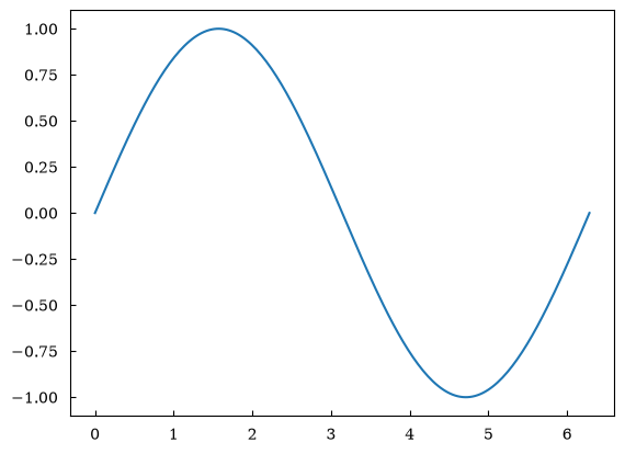

(<Figure size 640x480 with 1 Axes>, array([[<Axes: >]], dtype=object))

2 Multiple lines with labels, colors, and linestyles

canvas = Canvas()

canvas.plot(
    x, np.sin(x), label="sin(x)", color="royalblue", linestyle="solid", linewidth=2
)
canvas.plot(
    x, np.cos(x), label="cos(x)", color="tomato", linestyle="dashed", linewidth=2
)
canvas.plot(
    x,
    np.sin(2 * x),
    label="sin(2x)",
    color="forestgreen",
    linestyle="dotted",
    linewidth=1.5,
)

canvas.set_xlabel("x")
canvas.set_ylabel("y")
canvas.set_title("Sine and Cosine")
canvas.set_legend(True)

canvas.show(backend=BACKEND)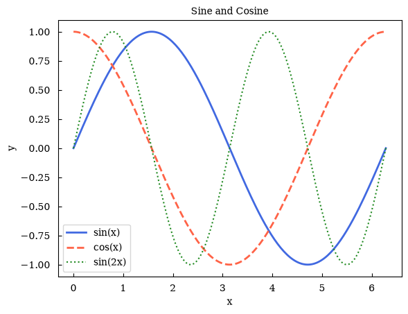

(<Figure size 640x480 with 1 Axes>,
 array([[<Axes: title={'center': 'Sine and Cosine'}, xlabel='x', ylabel='y'>]],
       dtype=object))

3 Canvas-level shortcut API

For single-subplot figures you can call plot methods directly on the Canvas object — they are forwarded to the subplot at row=0, col=0.

canvas = Canvas(ratio=0.5, fontsize=12)

canvas.plot(x, np.sin(x), label="sin(x)", color="steelblue")
canvas.plot(x, np.cos(x), label="cos(x)", color="darkorange", linestyle="dashed")

canvas.set_xlabel("angle (rad)")
canvas.set_ylabel("amplitude")
canvas.set_title("Using canvas-level methods")
canvas.set_legend(True)
canvas.set_grid(True)

canvas.show(backend=BACKEND)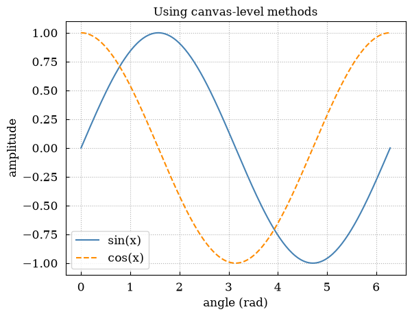

(<Figure size 640x480 with 1 Axes>,
 array([[<Axes: title={'center': 'Using canvas-level methods'}, xlabel='angle (rad)', ylabel='amplitude'>]],
       dtype=object))

4 Configuring the subplot at creation time

add_subplot() accepts convenience kwargs so you can set labels, grid, and legend in one call.

canvas = Canvas(ratio=0.5)
ax = canvas.add_subplot(
    title="Configured at creation",
    xlabel="x",
    ylabel="f(x)",
    grid=True,
    legend=True,
)

canvas.plot(x, np.sin(x), label="sin", color="royalblue")
canvas.plot(x, x / (2 * np.pi), label="x/2π", color="coral", linestyle="dashed")

canvas.show(backend=BACKEND)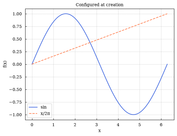

(<Figure size 640x480 with 1 Axes>,
 array([[<Axes: title={'center': 'Configured at creation'}, xlabel='x', ylabel='f(x)'>]],
       dtype=object))

5 Saving a figure

Use canvas.savefig() to write the figure to disk. The file extension determines the format; pass backend='matplotlib' for PDF output.

canvas = Canvas(ratio=0.5)
ax = canvas.add_subplot(xlabel="x", ylabel="sin(x)", grid=True)
canvas.plot(x, np.sin(x), color="steelblue")

canvas.savefig("tutorial_01_output.png")
print("Figure saved to tutorial_01_output.png")

Figure saved to tutorial_01_output.png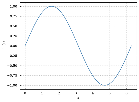

Summary

Task	Code
Create a canvas	canvas = Canvas()
Add a line	canvas.plot(x, y, label=..., color=..., linestyle=...)
Optional Matplotlib-style axes	canvas, ax = Canvas.subplots()
Labels / title	canvas.set_xlabel(), canvas.set_ylabel(), canvas.set_title()
Legend / grid	canvas.set_legend(True), canvas.set_grid(True)
Display	canvas.show()
Save	canvas.savefig('out.png')

Continue to Tutorial 02 to learn about multi-subplot layouts.