Plot types

Download notebookView on GitHubRun when the site was built.

maxplotlib exposes all common Matplotlib plot types through a unified API. This notebook demonstrates each type individually, then shows how to combine multiple types in a single subplot.

Plot types covered: plot · scatter · bar · fill_between · errorbar · axhline / axvline · hlines / vlines · combined plots · annotate / text

import numpy as np

from maxplotlib import Canvas

%matplotlib inline

rng = np.random.default_rng(42)
x = np.linspace(0, 2 * np.pi, 300)

Backend selection

All examples in this tutorial use the same Canvas API; you can switch rendering backends at any time:

• BACKEND = "matplotlib" for static Matplotlib output
• BACKEND = "plotly" for interactive Plotly output (Jupyter-friendly)

Most cells end with canvas.show(backend=BACKEND) so you can re-run the whole notebook with a different backend.

# Change to "plotly" for interactive output
BACKEND = "matplotlib"

1 Line plot — canvas.plot()

canvas = Canvas()

canvas.plot(
    x, np.sin(x), label="sin(x)", color="royalblue", linestyle="solid", linewidth=2
)
canvas.plot(
    x, np.cos(x), label="cos(x)", color="tomato", linestyle="dashed", linewidth=2
)

canvas.set_xlabel("x")
canvas.set_ylabel("y")
canvas.set_title("Line Plot")
canvas.set_legend(True)
canvas.set_grid(True)
canvas.show(backend=BACKEND)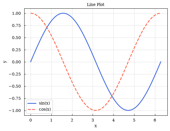

(<Figure size 640x480 with 1 Axes>,
 array([[<Axes: title={'center': 'Line Plot'}, xlabel='x', ylabel='y'>]],
       dtype=object))

2 Scatter plot — ax.scatter()

Use c= to colour each point by a scalar value (requires a colormap-compatible array).

n = 200
sx = rng.standard_normal(n)
sy = rng.standard_normal(n)
values = np.sqrt(sx**2 + sy**2)  # colour by distance from origin

canvas = Canvas()
canvas.scatter(sx, sy, c=values, s=30, label="data points")
canvas.set_xlabel("x")
canvas.set_ylabel("y")
canvas.set_title("Scatter Plot — coloured by distance")
canvas.set_aspect("equal")
canvas.show(backend=BACKEND)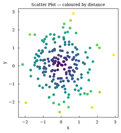

(<Figure size 640x480 with 1 Axes>,
 array([[<Axes: title={'center': 'Scatter Plot — coloured by distance'}, xlabel='x', ylabel='y'>]],
       dtype=object))

3 Bar chart — ax.bar()

categories = ["Jan", "Feb", "Mar", "Apr", "May", "Jun"]
values_bar = [12, 19, 15, 22, 30, 27]

canvas = Canvas()
canvas.bar(categories, values_bar, color="steelblue", width=0.6, label="monthly sales")
canvas.set_xlabel("Month")
canvas.set_ylabel("Sales (units)")
canvas.set_title("Bar Chart")
canvas.set_legend(True)
# canvas.show(backend=BACKEND) # TODO: Fix this error

4 Fill between — ax.fill_between()

Useful for shading confidence bands or uncertainty regions.

t = np.linspace(0, 4 * np.pi, 300)
mean = np.sin(t) * np.exp(-t / 10)
upper = mean + 0.3 * (1 - t / (4 * np.pi))
lower = mean - 0.3 * (1 - t / (4 * np.pi))

canvas = Canvas()
canvas.plot(t, mean, color="royalblue", label="mean", linewidth=2)
canvas.fill_between(t, lower, upper, alpha=0.25, color="royalblue", label="±1 std")
canvas.set_xlabel("t")
canvas.set_ylabel("value")
canvas.set_title("Fill Between — Confidence Band")
canvas.set_legend(True)
canvas.show(backend=BACKEND)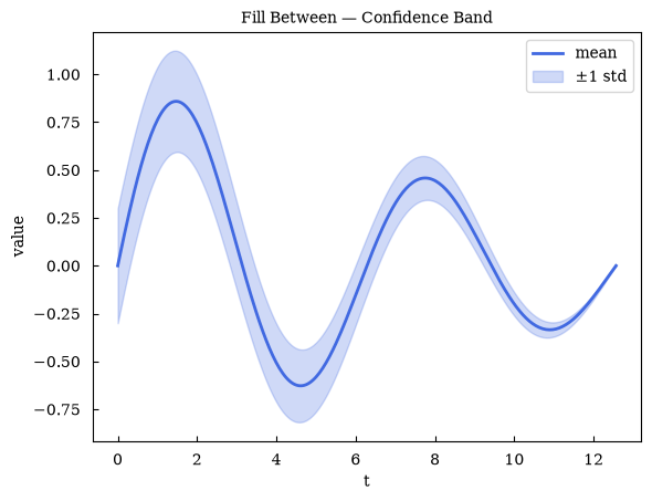

(<Figure size 640x480 with 1 Axes>,
 array([[<Axes: title={'center': 'Fill Between — Confidence Band'}, xlabel='t', ylabel='value'>]],
       dtype=object))

5 Error bars — ax.errorbar()

xm = np.linspace(0, 2 * np.pi, 12)
ym = np.sin(xm) + rng.normal(0, 0.1, len(xm))
yerr = 0.1 + 0.05 * rng.random(len(xm))

canvas = Canvas()
canvas.errorbar(
    xm, ym, yerr=yerr, fmt="o", capsize=4, color="tomato", label="measurements"
)
canvas.plot(x, np.sin(x), color="gray", linestyle="dashed", label="true sin(x)")
canvas.set_xlabel("x")
canvas.set_ylabel("y")
canvas.set_title("Error Bars")
canvas.set_legend(True)
canvas.set_grid(True)
canvas.show(backend=BACKEND)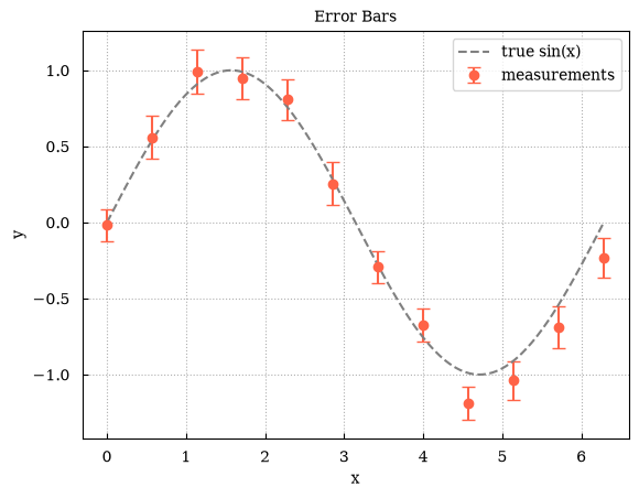

(<Figure size 640x480 with 1 Axes>,
 array([[<Axes: title={'center': 'Error Bars'}, xlabel='x', ylabel='y'>]],
       dtype=object))

6 Reference lines — axhline and axvline

Span the entire axis to mark thresholds or zero-crossings.

canvas = Canvas()
canvas.plot(x, np.sin(x), color="royalblue", label="sin(x)")

canvas.axhline(y=0, color="black", linestyle="solid", linewidth=0.8)
canvas.axhline(y=0.5, color="green", linestyle="dashed", linewidth=1.2, label="y = 0.5")
canvas.axhline(
    y=-0.5, color="green", linestyle="dashed", linewidth=1.2, label="y = -0.5"
)
canvas.axvline(x=np.pi, color="red", linestyle="dotted", linewidth=1.5, label="x = π")

canvas.set_xlabel("x")
canvas.set_title("axhline / axvline")
canvas.set_legend(True)
canvas.show(backend=BACKEND)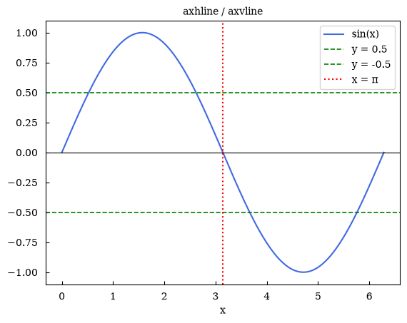

(<Figure size 640x480 with 1 Axes>,
 array([[<Axes: title={'center': 'axhline / axvline'}, xlabel='x'>]],
       dtype=object))

7 Segment lines — hlines and vlines

Draw multiple horizontal or vertical line segments with explicit start/end coordinates.

canvas = Canvas()
canvas.plot(x, np.sin(x), color="lightgray", linewidth=1)

# Horizontal segments spanning half the x-range
canvas.hlines(
    y=[0.5, -0.5],
    xmin=0,
    xmax=np.pi,
    colors="seagreen",
    linestyles="dashed",
    label="hlines at ±0.5",
)

# Vertical segments at specific x positions
canvas.vlines(
    x=[np.pi / 2, 3 * np.pi / 2],
    ymin=-1,
    ymax=1,
    colors="tomato",
    linestyles="dotted",
    label="vlines at π/2, 3π/2",
)

canvas.set_xlabel("x")
canvas.set_title("hlines / vlines")
canvas.set_legend(True)
canvas.show(backend=BACKEND)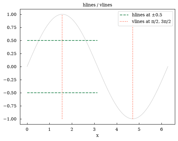

(<Figure size 640x480 with 1 Axes>,
 array([[<Axes: title={'center': 'hlines / vlines'}, xlabel='x'>]],
       dtype=object))

8 Combining plot types

A single subplot can hold many plot types simultaneously. Here we overlay a line, a shaded uncertainty band, and scatter points.

t = np.linspace(0, 2 * np.pi, 300)
signal = np.sin(t) * np.exp(-t / 8)
noise = rng.normal(0, 0.08, len(t))
band = 0.15 * np.exp(-t / 8)

# Sparse measurement points
tidx = np.arange(0, len(t), 20)
tx, ty = t[tidx], (signal + noise)[tidx]

canvas = Canvas()

canvas.fill_between(
    t, signal - band, signal + band, alpha=0.2, color="royalblue", label="uncertainty"
)
canvas.plot(t, signal, color="royalblue", linewidth=2, label="model")
canvas.scatter(tx, ty, color="tomato", s=25, marker="o", label="measurements")
canvas.axhline(y=0, color="gray", linestyle="dashed", linewidth=0.8)

canvas.set_xlabel("time")
canvas.set_ylabel("amplitude")
canvas.set_title("Combined: line + fill_between + scatter")
canvas.set_legend(True)
canvas.set_grid(True)
canvas.show(backend=BACKEND)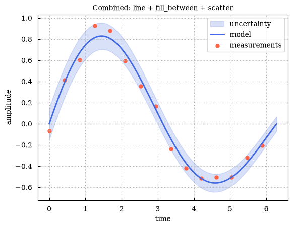

(<Figure size 640x480 with 1 Axes>,
 array([[<Axes: title={'center': 'Combined: line + fill_between + scatter'}, xlabel='time', ylabel='amplitude'>]],
       dtype=object))

9 Annotations — ax.annotate() and ax.text()

canvas = Canvas()
canvas.plot(x, np.sin(x), color="royalblue")

# Arrow annotation pointing to the peak
canvas.annotate(
    "peak",
    xy=(np.pi / 2, 1.0),
    xytext=(np.pi / 2 + 0.8, 0.7),
    arrowprops=dict(arrowstyle="->"),
)

# Free-floating text label
canvas.text(3 * np.pi / 2, 0.15, "zero\ncrossing", ha="center", fontsize=9)

canvas.set_xlabel("x")
canvas.set_ylabel("sin(x)")
canvas.set_title("Annotate and Text")
canvas.show(backend=BACKEND)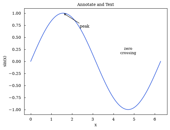

(<Figure size 640x480 with 1 Axes>,
 array([[<Axes: title={'center': 'Annotate and Text'}, xlabel='x', ylabel='sin(x)'>]],
       dtype=object))

Summary

Plot type	Method	Key kwargs
Line	canvas.plot(x, y)	color, linestyle, linewidth, label
Scatter	ax.scatter(x, y)	c, s, marker, label
Bar	ax.bar(x, height)	color, width, label
Filled band	ax.fill_between(x, y1, y2)	alpha, color, label
Error bars	ax.errorbar(x, y, yerr=...)	fmt, capsize, label
Full-span h/v line	ax.axhline(y=...) / ax.axvline(x=...)	color, linestyle
Segment lines	ax.hlines(y, xmin, xmax) / ax.vlines(x, ymin, ymax)	colors, linestyles
Arrow annotation	ax.annotate(text, xy=..., xytext=..., arrowprops=...)
Free text	ax.text(x, y, text)	ha, fontsize

You now know the full set of plot types available in maxplotlib. 🎉