Axes and annotations

Download notebook View on GitHubRun when the site was built.

This tutorial covers every way to control the coordinate frame of a subplot: labels, limits, tick marks, log scales, grids, legends, and annotations.

import numpy as np

from maxplotlib import Canvas

Backend selection

All examples in this tutorial use the same Canvas API; you can switch rendering backends at any time:

BACKEND = "matplotlib" for static Matplotlib output
BACKEND = "plotly" for interactive Plotly output (Jupyter-friendly)

Most cells end with canvas.show(backend=BACKEND) so you can re-run the whole notebook with a different backend.

# Change to "plotly" for interactive output
BACKEND = "matplotlib"

1 · Labels and title

LaTeX strings are supported in all text arguments.

x = np.linspace(0, 2 * np.pi, 200)

canvas = Canvas(width="10cm", ratio=0.55)
canvas.plot(x, np.sin(x), color="steelblue")

canvas.set_xlabel(r"$x$ (radians)")
canvas.set_ylabel(r"$\sin(x)$")
canvas.set_title(r"The sine function $f(x) = \sin(x)$")
canvas.show(backend=BACKEND)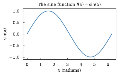

(<Figure size 393.701x216.535 with 1 Axes>,
 array([[<Axes: title={'center': 'The sine function $f(x) = \\sin(x)$'}, xlabel='$x$ (radians)', ylabel='$\\sin(x)$'>]],
       dtype=object))

2 · Axis limits

x = np.linspace(0, 4 * np.pi, 300)

canvas = Canvas(width="10cm", ratio=0.5)
canvas.plot(x, np.sin(x), color="tomato")

# Show only the first full period
canvas.set_xlim(0, 2 * np.pi)
canvas.set_ylim(-1.2, 1.2)

canvas.set_xlabel("x")
canvas.set_ylabel(r"$\sin(x)$")
canvas.set_title("Axis limits: first period only")
canvas.show(backend=BACKEND)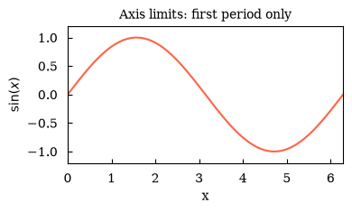

(<Figure size 393.701x196.85 with 1 Axes>,
 array([[<Axes: title={'center': 'Axis limits: first period only'}, xlabel='x', ylabel='$\\sin(x)$'>]],
       dtype=object))

3 · Custom ticks

Pass tick positions and optional labels to set_xticks.

months = [
    "Jan",
    "Feb",
    "Mar",
    "Apr",
    "May",
    "Jun",
    "Jul",
    "Aug",
    "Sep",
    "Oct",
    "Nov",
    "Dec",
]
temps = [3, 4, 7, 12, 17, 21, 23, 22, 18, 13, 7, 4]

canvas = Canvas(width="12cm", ratio=0.45)
canvas.plot(range(12), temps, marker="o", color="steelblue", linewidth=2)

canvas.set_xticks(list(range(12)), labels=months)
canvas.set_ylabel(r"Temperature ($^\circ$C)")
canvas.set_title("Monthly average temperature")
canvas.show(backend=BACKEND)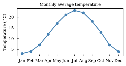

(<Figure size 472.441x212.598 with 1 Axes>,
 array([[<Axes: title={'center': 'Monthly average temperature'}, ylabel='Temperature ($^\\circ$C)'>]],
       dtype=object))

4 · Log scale

Use set_yscale('log') for data spanning several orders of magnitude. Compare linear and log in a 1×2 layout.

x = np.linspace(0.1, 5, 200)
y = np.exp(2 * x)

canvas, (ax1, ax2) = Canvas.subplots(ncols=2, width="14cm", ratio=0.4)

ax1.plot(x, y, color="seagreen")
ax1.set_xlabel("x")
ax1.set_ylabel(r"$e^{2x}$")
ax1.set_title("Linear scale")

ax2.plot(x, y, color="seagreen")
ax2.set_xlabel("x")
ax2.set_yscale("log")
ax2.set_title("Log scale")

canvas.suptitle("Linear vs log scale")
canvas.show(backend=BACKEND)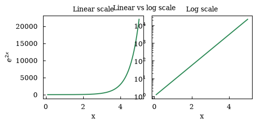

(<Figure size 551.181x220.472 with 2 Axes>,
 array([[<Axes: title={'center': 'Linear scale'}, xlabel='x', ylabel='$e^{2x}$'>,
         <Axes: title={'center': 'Log scale'}, xlabel='x'>]], dtype=object))

5 · Grid

x = np.linspace(0, 2 * np.pi, 200)

canvas, (ax1, ax2) = Canvas.subplots(ncols=2, width="12cm", ratio=0.5)

ax1.plot(x, np.cos(x), color="steelblue")
ax1.set_title("No grid")
ax1.set_xlabel("x")

ax2.plot(x, np.cos(x), color="steelblue")
ax2.set_grid(True)
ax2.set_title("With grid")
ax2.set_xlabel("x")

canvas.show(backend=BACKEND)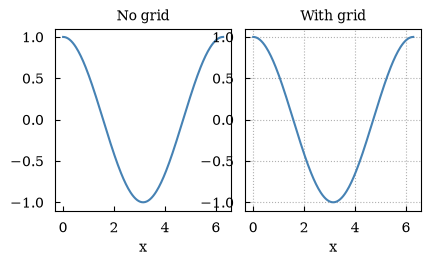

(<Figure size 472.441x236.22 with 2 Axes>,
 array([[<Axes: title={'center': 'No grid'}, xlabel='x'>,
         <Axes: title={'center': 'With grid'}, xlabel='x'>]], dtype=object))

6 · Legend

Enable with set_legend(True). Labels come from label= kwargs.

x = np.linspace(0, 2 * np.pi, 200)

canvas = Canvas(width="10cm", ratio=0.55)
canvas.plot(x, np.sin(x), color="steelblue", label=r"$\sin(x)$")
canvas.plot(x, np.cos(x), color="tomato", label=r"$\cos(x)$")
canvas.plot(x, np.sin(2 * x), color="seagreen", label=r"$\sin(2x)$", linestyle="dashed")

canvas.set_xlabel("x")
canvas.set_legend(True)
canvas.set_title("Legend demo")
canvas.show(backend=BACKEND)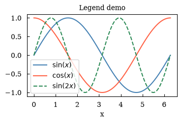

(<Figure size 393.701x216.535 with 1 Axes>,
 array([[<Axes: title={'center': 'Legend demo'}, xlabel='x'>]],
       dtype=object))

7 · annotate

Draw an arrow from a text label to a data point.

x = np.linspace(0, 2 * np.pi, 200)
y = np.sin(x)

canvas = Canvas(width="10cm", ratio=0.55)
canvas.plot(x, y, color="steelblue")

# Annotate the maximum
canvas.annotate(
    r"maximum $\approx 1$",
    xy=(np.pi / 2, 1.0),
    xytext=(np.pi / 2 + 1.0, 0.7),
    arrowprops=dict(arrowstyle="->", color="black"),
    fontsize=9,
    color="darkred",
)

canvas.set_xlabel("x")
canvas.set_ylabel(r"$\sin(x)$")
canvas.set_title("annotate demo")
canvas.show(backend=BACKEND)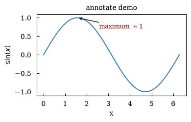

(<Figure size 393.701x216.535 with 1 Axes>,
 array([[<Axes: title={'center': 'annotate demo'}, xlabel='x', ylabel='$\\sin(x)$'>]],
       dtype=object))

8 · text

Place a text label at arbitrary data coordinates.

x = np.linspace(-2, 2, 200)

canvas = Canvas(width="10cm", ratio=0.55)
canvas.plot(x, x**2, color="darkorange")

canvas.text(
    0, 3.2, r"$f(x) = x^2$", ha="center", va="bottom", fontsize=12, color="darkorange"
)

canvas.set_xlabel("x")
canvas.set_ylabel(r"$f(x)$")
canvas.set_title("text demo")
canvas.show(backend=BACKEND)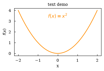

(<Figure size 393.701x216.535 with 1 Axes>,
 array([[<Axes: title={'center': 'text demo'}, xlabel='x', ylabel='$f(x)$'>]],
       dtype=object))

9 · Aspect ratio

set_aspect('equal') ensures a circle looks circular.

theta = np.linspace(0, 2 * np.pi, 300)

canvas = Canvas(width="7cm", ratio=1.0)
canvas.plot(np.cos(theta), np.sin(theta), color="steelblue", linewidth=2)
canvas.set_aspect("equal")
canvas.set_title("Circle with equal aspect ratio")
canvas.set_xlabel("x")
canvas.set_ylabel("y")
canvas.show(backend=BACKEND)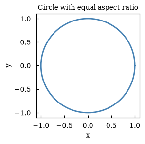

(<Figure size 275.591x275.591 with 1 Axes>,
 array([[<Axes: title={'center': 'Circle with equal aspect ratio'}, xlabel='x', ylabel='y'>]],
       dtype=object))

Summary

Method	Purpose
`set_xlabel` / `set_ylabel`	Axis labels (LaTeX OK)
`set_title`	Subplot title
`set_xlim` / `set_ylim`	Axis range
`set_xticks(pos, labels=)`	Custom tick marks
`set_yscale('log')`	Logarithmic scale
`set_grid(True)`	Background grid
`set_legend(True)`	Auto legend
`annotate(...)`	Arrow annotation
`text(x, y, s)`	Free text label
`set_aspect('equal')`	Equal x/y scaling

Part of the max-models projects Source on GitHub