Styling

Download notebookView on GitHubRun when the site was built.

maxplotlib passes matplotlib kwargs directly to the underlying renderer, so every colour, linestyle, marker, and alpha option you know from matplotlib works here too.

import numpy as np

from maxplotlib import Canvas

Backend selection

All examples in this tutorial use the same Canvas API; you can switch rendering backends at any time:

• BACKEND = "matplotlib" for static Matplotlib output
• BACKEND = "plotly" for interactive Plotly output (Jupyter-friendly)

Most cells end with canvas.show(backend=BACKEND) so you can re-run the whole notebook with a different backend.

# Change to "plotly" for interactive output
BACKEND = "matplotlib"

1 · Colors

Named colors, hex strings, and RGB tuples are all accepted.

x = np.linspace(0, 2 * np.pi, 200)

canvas = Canvas(width="10cm", ratio=0.6)

canvas.plot(x, np.sin(x), color="steelblue", label="named: steelblue")
canvas.plot(x, np.sin(x - 0.5), color="#e74c3c", label="hex: #e74c3c")
canvas.plot(x, np.sin(x - 1.0), color=(0.2, 0.7, 0.3), label="RGB tuple")

canvas.set_xlabel("x")
canvas.set_ylabel("y")
canvas.set_title("Color options")
canvas.set_legend(True)
canvas.show(backend=BACKEND)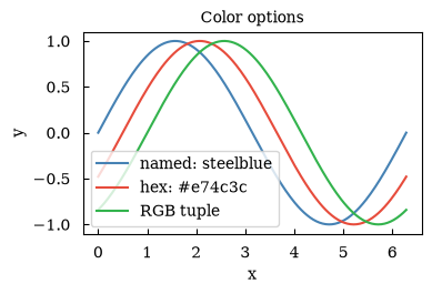

(<Figure size 393.701x236.22 with 1 Axes>,
 array([[<Axes: title={'center': 'Color options'}, xlabel='x', ylabel='y'>]],
       dtype=object))

2 · Linestyles

Use long names ('solid', 'dashed', 'dotted', 'dashdot') or short aliases ('-', '--', ':', '-.').

x = np.linspace(0, 4 * np.pi, 300)
styles = [("solid", "-"), ("dashed", "--"), ("dotted", ":"), ("dashdot", "-.")]

canvas = Canvas(width="10cm", ratio=0.6)

for i, (name, ls) in enumerate(styles):
    canvas.plot(
        x,
        np.sin(x) + i * 0.4,
        linestyle=ls,
        linewidth=2,
        color="steelblue",
        label=f"{name!r} / {ls!r}",
    )

canvas.set_xlabel("x")
canvas.set_title("Linestyle comparison")
canvas.set_legend(True)
canvas.show(backend=BACKEND)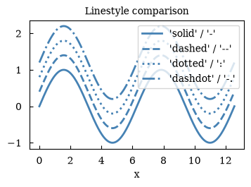

(<Figure size 393.701x236.22 with 1 Axes>,
 array([[<Axes: title={'center': 'Linestyle comparison'}, xlabel='x'>]],
       dtype=object))

3 · Markers

Pass marker= to ax.plot or ax.scatter.

x = np.linspace(0, 2 * np.pi, 10)
markers = ["o", "s", "^", "D", "*", "x", "+"]

canvas = Canvas(width="10cm", ratio=0.65)

for i, m in enumerate(markers):
    canvas.plot(
        x,
        np.sin(x) + i * 0.5,
        marker=m,
        linestyle="-",
        markersize=7,
        label=f"marker={m!r}",
    )

canvas.set_xlabel("x")
canvas.set_title("Marker comparison")
canvas.set_legend(True)
canvas.show(backend=BACKEND)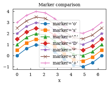

(<Figure size 393.701x255.906 with 1 Axes>,
 array([[<Axes: title={'center': 'Marker comparison'}, xlabel='x'>]],
       dtype=object))

4 · Linewidth and markersize

Control visual weight with linewidth= and markersize=.

x = np.linspace(0, 2 * np.pi, 40)

canvas = Canvas(width="10cm", ratio=0.55)

canvas.plot(x, np.sin(x), linewidth=0.8, marker="o", markersize=3, label="thin / small")
canvas.plot(x, np.sin(x) - 0.6, linewidth=2.5, marker="o", markersize=7, label="medium")
canvas.plot(
    x, np.sin(x) - 1.2, linewidth=4.5, marker="o", markersize=12, label="thick / large"
)

canvas.set_xlabel("x")
canvas.set_title("Linewidth and markersize")
canvas.set_legend(True)
canvas.show(backend=BACKEND)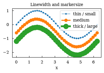

(<Figure size 393.701x216.535 with 1 Axes>,
 array([[<Axes: title={'center': 'Linewidth and markersize'}, xlabel='x'>]],
       dtype=object))

5 · Alpha (transparency)

alpha= ranges from 0 (invisible) to 1 (opaque). Useful for overlapping fill_between regions.

x = np.linspace(0, 2 * np.pi, 200)

canvas = Canvas(width="10cm", ratio=0.55)

canvas.fill_between(x, np.sin(x), 0, alpha=0.7, color="steelblue", label="alpha=0.7")
canvas.fill_between(x, np.sin(2 * x), 0, alpha=0.4, color="tomato", label="alpha=0.4")
canvas.fill_between(x, np.sin(3 * x), 0, alpha=0.2, color="seagreen", label="alpha=0.2")

canvas.set_xlabel("x")
canvas.set_title("Alpha transparency")
canvas.set_legend(True)
canvas.show(backend=BACKEND)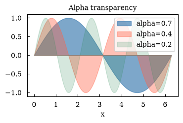

(<Figure size 393.701x216.535 with 1 Axes>,
 array([[<Axes: title={'center': 'Alpha transparency'}, xlabel='x'>]],
       dtype=object))

6 · Combining styles – a publication-ready plot

Combine color, linestyle, marker, linewidth, and alpha in one plot.

x = np.linspace(0, 2 * np.pi, 80)
noise = np.random.default_rng(0).normal(0, 0.05, len(x))

canvas = Canvas(width="10cm", ratio=0.6)

# Shaded uncertainty band
canvas.fill_between(
    x, np.sin(x) - 0.15, np.sin(x) + 0.15, alpha=0.15, color="steelblue"
)

# Noisy data
canvas.scatter(
    x, np.sin(x) + noise, color="steelblue", marker="o", s=18, alpha=0.6, label="data"
)

# Clean model
canvas.plot(
    x,
    np.sin(x),
    color="#e74c3c",
    linestyle="dashed",
    linewidth=2.0,
    alpha=0.9,
    label="model",
)

canvas.set_xlabel("x")
canvas.set_ylabel("y")
canvas.set_title("Publication-style plot")
canvas.set_legend(True)
canvas.show(backend=BACKEND)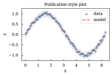

(<Figure size 393.701x236.22 with 1 Axes>,
 array([[<Axes: title={'center': 'Publication-style plot'}, xlabel='x', ylabel='y'>]],
       dtype=object))

Summary

Option	Example
Named color	color='steelblue'
Hex color	color='#e74c3c'
RGB tuple	color=(0.2, 0.7, 0.3)
Linestyle	linestyle='dashed' or '--'
Marker	marker='o'
Linewidth	linewidth=2.0
Markersize	markersize=7
Transparency	alpha=0.5