Quickstart

A Canvas holds the figure: its subplots, lines and styling, independent of how it is drawn. The backend is chosen when you render it.

import numpy as np
from maxplotlib import Canvas

x = np.linspace(0, 2 * np.pi, 200)
y = np.sin(x)

canvas, ax = Canvas.subplots()
ax.plot(x, y)

Plot the figure with the default (Matplotlib) backend:

canvas.show()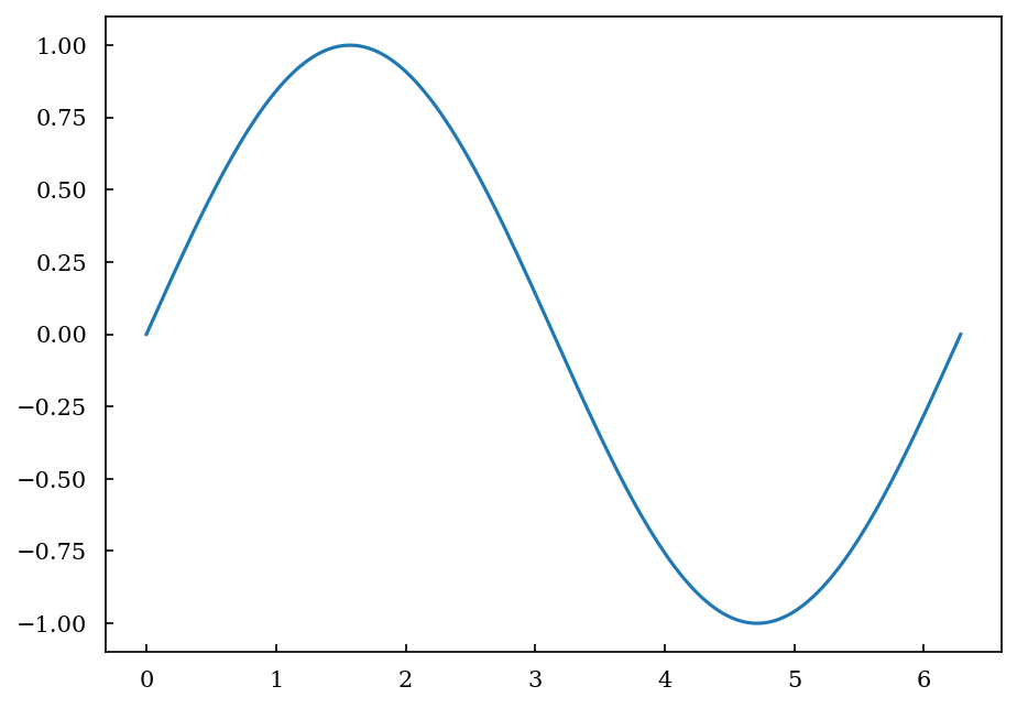

Use canvas.plot(x, y) to add data directly to a canvas. When you want to explicitly render an already-built canvas, use canvas.render(...). The older canvas.plot(backend=...) spelling is still supported for compatibility, but emits a FutureWarning.

Add several lines at once with shared styling:

canvas.plot_many(
    [(x, np.sin(x)), (x, np.cos(x))],
    labels=["sin(x)", "cos(x)"],
    linewidth=2,
)

Other backends

The same canvas renders with every backend:

canvas.show(backend="plotly")  # an interactive Plotly figure
canvas.show(backend="plotext")  # a plot in the terminal
canvas.savefig("sine.pdf", backend="tikzfigure")  # TikZ code, compiled with LaTeX

savefig picks the format from the file name: whatever Matplotlib writes (PNG, PDF, SVG, …); HTML for Plotly (include_plotlyjs="cdn" for a small file that loads plotly.js from a CDN), or an image with kaleido; a text file for plotext; and .tikz, .tex, PDF or PNG for TikZ (PDF and PNG compiled with LaTeX).

Next

The tutorials go through subplots, plot types, styling, axes and annotations, layers, each backend in detail, Gantt and flame charts, and xarray data. An existing Matplotlib figure can be imported with Canvas.from_matplotlib; see Matplotlib import.