Axis and layout

Download notebookView on GitHubRun when the site was built.

This tutorial demonstrates the latest Matplotlib-style wrappers: filled polygons, logarithmic shortcuts, axis limits and autoscaling, secondary axes, box aspect, and explicit tick labels.

import numpy as np

from maxplotlib import Canvas

x = np.linspace(0.1, 10, 200)

Filled polygons

fill() forwards polygon coordinates to Matplotlib and becomes a filled Plotly scatter trace.

canvas = Canvas()
canvas.fill([0, 1, 2, 1], [0, 2, 0, -1], color="tab:orange", alpha=0.5)
canvas.set_title("A filled polygon")
canvas.show()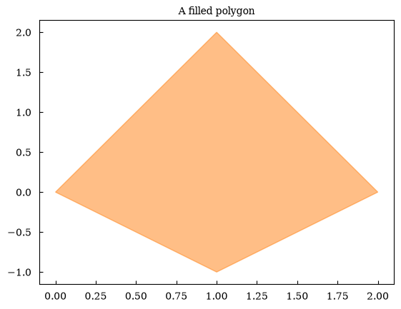

(<Figure size 640x480 with 1 Axes>,
 array([[<Axes: title={'center': 'A filled polygon'}>]], dtype=object))

Logarithmic plotting shortcuts

Use semilogx(), semilogy(), or loglog() when the data and axis scale should be configured together. The three-panel example below shows the optional fig/axs style for users familiar with Matplotlib; ordinary one-panel examples use Canvas directly.

canvas, (ax1, ax2, ax3) = Canvas.subplots(nrows=1, ncols=3)
ax1.semilogx(x, np.sin(x) + 2)
ax2.semilogy(x, np.exp(x / 4))
ax3.loglog(x, x**2)
ax1.set_title("semilogx")
ax2.set_title("semilogy")
ax3.set_title("loglog")
canvas.show()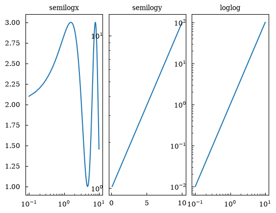

(<Figure size 640x480 with 3 Axes>,
 array([[<Axes: title={'center': 'semilogx'}>,
         <Axes: title={'center': 'semilogy'}>,
         <Axes: title={'center': 'loglog'}>]], dtype=object))

Axis limits, modes, and autoscaling

axis() accepts Matplotlib-style modes such as "equal", "tight", and "off", or a four-value [xmin, xmax, ymin, ymax] limit list. relim() and autoscale_view() recompute the visible limits from plotted data.

canvas = Canvas()
canvas.plot([0, 1, 2], [0, 4, 1])
canvas.axis([0, 2, -1, 5])
canvas.relim()
canvas.autoscale_view(tight=True)
canvas.show()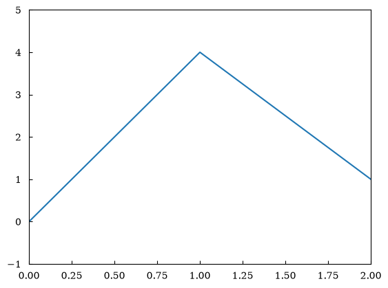

(<Figure size 640x480 with 1 Axes>, array([[<Axes: >]], dtype=object))

Secondary x- and y-axes

Secondary axes use forward and inverse functions. They are currently rendered by the Matplotlib backend.

canvas = Canvas()
canvas.plot(x, x**2)
canvas.set_xlabel("distance (m)")
canvas.set_ylabel("area (m²)")
canvas.secondary_xaxis(
    "top",
    functions=(lambda value: value / 1000, lambda value: value * 1000),
    label="distance (km)",
)
canvas.secondary_yaxis(
    "right",
    # the margin below 0 of the area axis has no length
    functions=(lambda value: np.sqrt(np.clip(value, 0, None)), lambda value: value**2),
    label="length (m)",
)
canvas.show()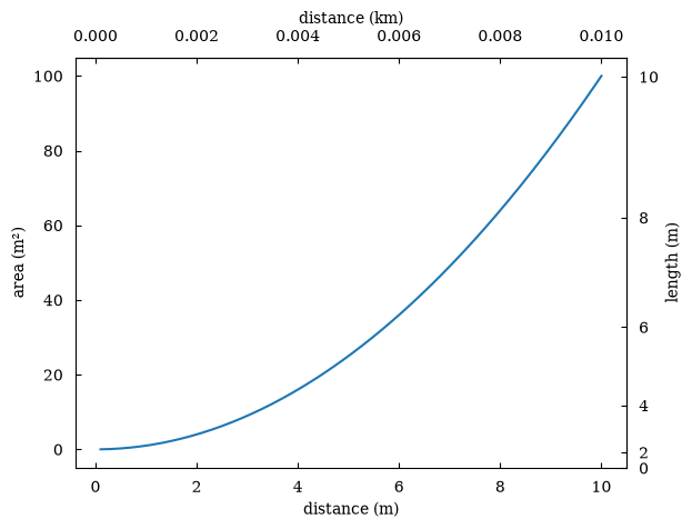

(<Figure size 640x480 with 1 Axes>,
 array([[<Axes: xlabel='distance (m)', ylabel='area (m²)'>]], dtype=object))

Box aspect and explicit tick labels

canvas = Canvas()
canvas.plot([0, 1, 2], [0, 1, 0], marker="o")
canvas.set_box_aspect(1)
canvas.set_xticks([0, 1, 2])
canvas.set_xticklabels(["start", "middle", "end"], rotation=25, color="navy")
canvas.set_yticks([0, 1])
canvas.set_yticklabels(["low", "high"], fontweight="bold")
canvas.show()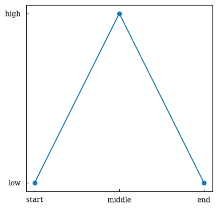

(<Figure size 640x480 with 1 Axes>, array([[<Axes: >]], dtype=object))

Plotly rendering

The filled polygon, logarithmic scales, axis modes, box aspect, and tick labels also work with Plotly. Secondary axes currently require Matplotlib.

plotly_canvas = Canvas()
plotly_canvas.fill(x, np.sin(x) + 2, color="purple", alpha=0.25)
plotly_canvas.loglog(x, x**2, color="black")
plotly_canvas.set_xticklabels(["small", "medium", "large"], color="darkgreen")
plotly_canvas.show(backend="plotly")