Flame charts

Download notebook View on GitHubRun when the site was built.

This tutorial demonstrates how to create flame charts using maxplotlib across different backends.

Flame charts are powerful visualizations for hierarchical profiling data, showing function call stacks and their execution times or sample counts.

from maxplotlib import Canvas

Basic Flame Chart

Let’s create a simple flame chart showing a function call hierarchy.

# Define function call hierarchy
labels = [
    "main()",  # 0 - root
    "process_data()",  # 1 - child of main
    "load_file()",  # 2 - child of process_data
    "parse_json()",  # 3 - child of process_data
    "validate()",  # 4 - child of process_data
]

# Parent indices (None for root, index for parent)
parents = [None, 0, 1, 1, 1]

# Duration or sample count for each function
values = [100, 60, 15, 20, 25]

# Start times (when each function begins)
start_times = [0, 0, 0, 15, 35]

# Create canvas and add flame chart
canvas = Canvas(nrows=1, ncols=1, figsize=(12, 6))
canvas.flame_chart(
    labels=labels,
    parents=parents,
    values=values,
    start_times=start_times,
    colormap="viridis",
    edgecolor="black",
)

canvas.set_xlabel("Time (ms)")
canvas.set_ylabel("Stack Depth")
canvas.set_title("Function Call Hierarchy")
canvas.render(backend="matplotlib")

(<Figure size 1200x600 with 1 Axes>,
 array([[<Axes: title={'center': 'Function Call Hierarchy'}, xlabel='Time (ms)', ylabel='Stack Depth'>]],
       dtype=object))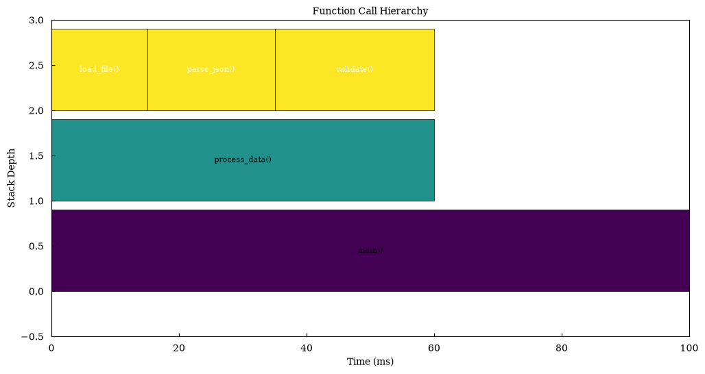

Complex Call Stack

Visualize a more complex profiling scenario with multiple levels.

# More complex hierarchy
labels = [
    "main()",
    "init()",
    "setup_db()",
    "connect()",
    "authenticate()",
    "process()",
    "fetch_data()",
    "query_db()",
    "transform()",
    "map()",
    "reduce()",
    "cleanup()",
]

parents = [
    None,  # main
    0,  # init -> main
    1,  # setup_db -> init
    2,  # connect -> setup_db
    2,  # authenticate -> setup_db
    0,  # process -> main
    5,  # fetch_data -> process
    6,  # query_db -> fetch_data
    5,  # transform -> process
    8,  # map -> transform
    8,  # reduce -> transform
    0,  # cleanup -> main
]

values = [200, 40, 30, 15, 15, 120, 50, 40, 70, 35, 35, 20]
start_times = [0, 0, 0, 0, 15, 40, 40, 40, 90, 90, 125, 180]

canvas = Canvas(nrows=1, ncols=1, figsize=(14, 8))
canvas.flame_chart(
    labels=labels,
    parents=parents,
    values=values,
    start_times=start_times,
    colormap="plasma",
    edgecolor="black",
)

canvas.set_xlabel("Time (ms)")
canvas.set_ylabel("Stack Depth")
canvas.set_title("Complex Application Profiling")
canvas.render(backend="matplotlib")

(<Figure size 1400x800 with 1 Axes>,
 array([[<Axes: title={'center': 'Complex Application Profiling'}, xlabel='Time (ms)', ylabel='Stack Depth'>]],
       dtype=object))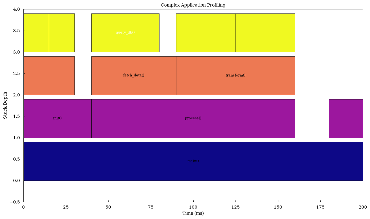

CPU Profiling Simulation

Simulate CPU profiling data with multiple parallel execution paths.

# Simulate CPU profiling with parallel tasks
labels = [
    "app_main",
    "worker_1",
    "compute_heavy",
    "math_ops",
    "worker_2",
    "io_bound",
    "read_file",
    "worker_3",
    "network_call",
    "http_request",
]

parents = [None, 0, 1, 2, 0, 4, 5, 0, 7, 8]
values = [150, 50, 40, 30, 45, 35, 25, 55, 45, 35]
start_times = [0, 0, 0, 5, 50, 50, 55, 95, 95, 100]

canvas = Canvas(nrows=1, ncols=1, figsize=(12, 6))
canvas.flame_chart(
    labels=labels,
    parents=parents,
    values=values,
    start_times=start_times,
    colormap="inferno",
    edgecolor="darkred",
)

canvas.set_xlabel("Time (ms)")
canvas.set_ylabel("Call Stack Depth")
canvas.set_title("CPU Profiling: Parallel Workers")
canvas.render(backend="matplotlib")

(<Figure size 1200x600 with 1 Axes>,
 array([[<Axes: title={'center': 'CPU Profiling: Parallel Workers'}, xlabel='Time (ms)', ylabel='Call Stack Depth'>]],
       dtype=object))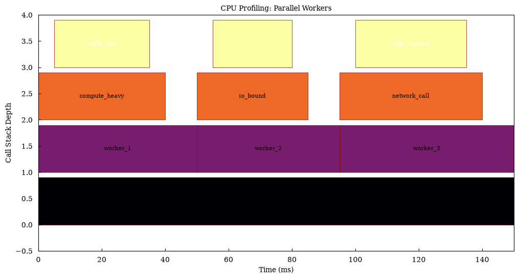

Interactive Flame Chart with Plotly

Create an interactive version for detailed exploration.

labels = [
    "main()",
    "process_data()",
    "load_file()",
    "parse_json()",
    "validate()",
    "compute()",
    "algorithm_a()",
    "algorithm_b()",
    "save_results()",
]

parents = [None, 0, 1, 1, 1, 0, 5, 5, 0]
values = [100, 40, 10, 15, 15, 50, 25, 25, 10]
start_times = [0, 0, 0, 10, 25, 40, 40, 65, 90]

canvas = Canvas(nrows=1, ncols=1, figsize=(12, 6))
canvas.flame_chart(
    labels=labels,
    parents=parents,
    values=values,
    start_times=start_times,
    colormap="Viridis",
    edgecolor="black",
)

canvas.set_xlabel("Time (ms)")
canvas.set_ylabel("Stack Depth")
canvas.set_title("Interactive Flame Chart - Hover for Details")
fig = canvas.render(backend="plotly")
fig.show()

Auto-computed Start Times

Let maxplotlib compute start times automatically from the hierarchy.

# When start_times=None, they are computed automatically
labels = ["root", "child1", "child2", "grandchild1", "grandchild2"]
parents = [None, 0, 0, 1, 1]
values = [100, 50, 50, 25, 25]

canvas = Canvas(nrows=1, ncols=1, figsize=(10, 5))
canvas.flame_chart(
    labels=labels,
    parents=parents,
    values=values,
    start_times=None,  # Auto-computed
    colormap="coolwarm",
)

canvas.set_xlabel("Relative Time")
canvas.set_ylabel("Depth")
canvas.set_title("Flame Chart with Auto-computed Start Times")
canvas.render(backend="matplotlib")

(<Figure size 1000x500 with 1 Axes>,
 array([[<Axes: title={'center': 'Flame Chart with Auto-computed Start Times'}, xlabel='Relative Time', ylabel='Depth'>]],
       dtype=object))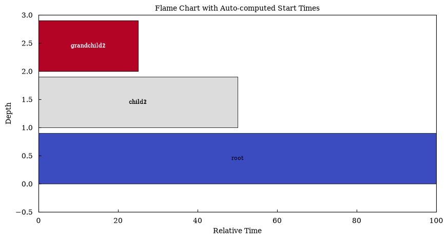

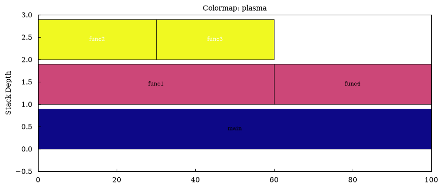
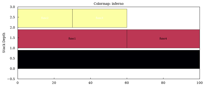
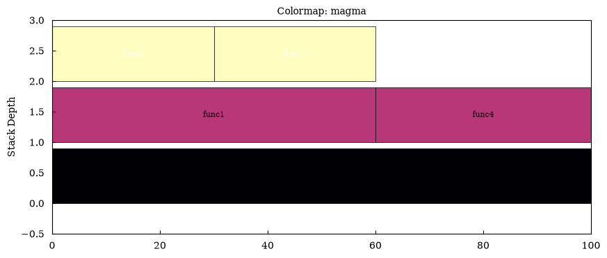
Comparison: Different Colormaps

Explore different colormap options for flame charts.

labels = ["main", "func1", "func2", "func3", "func4"]
parents = [None, 0, 1, 1, 0]
values = [100, 60, 30, 30, 40]
start_times = [0, 0, 0, 30, 60]

colormaps = ["viridis", "plasma", "inferno", "magma"]

for cmap in colormaps:
    canvas = Canvas(nrows=1, ncols=1, figsize=(10, 4))
    canvas.flame_chart(
        labels=labels,
        parents=parents,
        values=values,
        start_times=start_times,
        colormap=cmap,
        edgecolor="black",
    )
    canvas.set_title(f"Colormap: {cmap}")
    canvas.render(backend="matplotlib")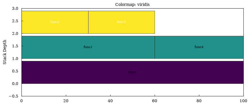

Real-world Example: Web Request Processing

Visualize the processing of a web request through various layers.

labels = [
    "handle_request",
    "authenticate",
    "check_token",
    "verify_signature",
    "route_handler",
    "validate_input",
    "business_logic",
    "db_query",
    "cache_check",
    "serialize_response",
    "json_encode",
    "send_response",
]

parents = [None, 0, 1, 2, 0, 4, 4, 6, 6, 0, 9, 0]
values = [200, 30, 20, 15, 140, 15, 100, 50, 30, 20, 15, 10]
start_times = [0, 0, 5, 10, 30, 30, 45, 45, 95, 170, 170, 190]

canvas = Canvas(nrows=1, ncols=1, figsize=(14, 7))
canvas.flame_chart(
    labels=labels,
    parents=parents,
    values=values,
    start_times=start_times,
    colormap="RdYlGn_r",
    edgecolor="black",
)

canvas.set_xlabel("Time (ms)")
canvas.set_ylabel("Call Stack")
canvas.set_title("Web Request Processing Profile")
canvas.render(backend="matplotlib")

(<Figure size 1400x700 with 1 Axes>,
 array([[<Axes: title={'center': 'Web Request Processing Profile'}, xlabel='Time (ms)', ylabel='Call Stack'>]],
       dtype=object))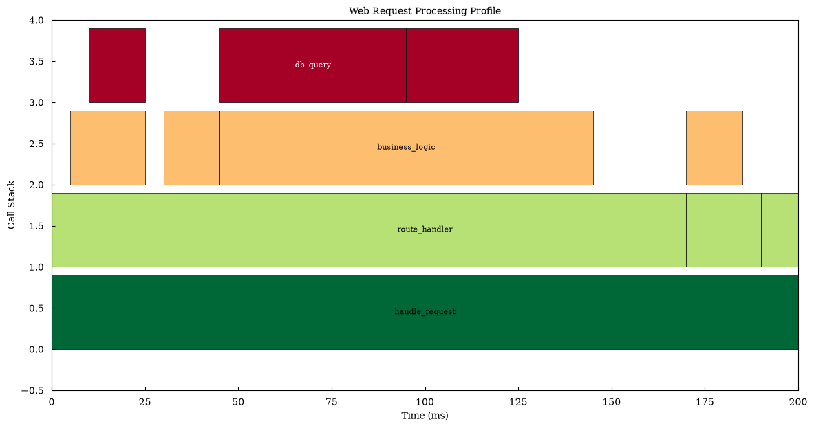

Summary

Flame charts in maxplotlib support:

Hierarchical profiling data visualization
Automatic depth calculation from parent relationships
Optional auto-computed start times
Multiple colormap options
All backends: matplotlib, plotly, plotext, tikzfigure
Interactive exploration with plotly backend
Customizable colors and edge styling

Perfect for:

CPU profiling analysis
Function call stack visualization
Performance bottleneck identification
Execution time analysis

Part of the max-models projects Source on GitHub