Getting started
A field on a uniform grid: create it, fill it, evaluate it, plot it and compute with it.
A Field is a grid from simgeometry plus the values on its nodes, one or several components
per node. This page goes through the basic operations on one process; the
MPI and halos example splits the same fields over several.
import numpy as npimport plasma_plots  # noqa: F401  (registers the .plasma accessor on xarray)
from mpifield import Field
A field on a grid
Section titled “A field on a grid”num_gridpoints nodes span lower_bound to upper_bound along each axis, so the spacing is
(upper - lower) / (n - 1). A field starts at zero; get_grid_points gives the node
coordinates of each axis.
phi = Field( ndim=2, lower_bound=(0.0, 0.0), upper_bound=(0.1, 0.05), num_gridpoints=(101, 51),)x, y = np.meshgrid(*phi.get_grid_points(), indexing="ij")print(phi)print("spacing:", phi.grid_spacing)Field(ndim=2, num_gridpoints=(101, 51), num_components=1, lower_bound=(0.0, 0.0), upper_bound=(0.1, 0.05), distributed=False)rank 0: stored block (101, 51, 1), index bounds [(0, 101), (0, 51)]spacing: [0.001 0.001]set_field_data takes a scalar, an array of the grid’s shape (for a scalar field or one
component) or of the full shape num_gridpoints + (num_components,).
phi.set_field_data(1000.0 * np.exp(-((x - 0.05) ** 2 + (y - 0.025) ** 2) / 1e-4))print(phi.max(), phi.sum())1000.0 314062.79166152334Evaluating and plotting
Section titled “Evaluating and plotting”evaluate returns an xarray.DataArray: the nodes as they are, or interpolated on a line, a
plane or scattered points. A scalar fixes a coordinate. plot draws the same with
plasma-plots: a line for one free coordinate,
a map for two.
profile = phi.evaluate(y=0.025, name="phi", units="V")profile<xarray.DataArray 'phi' (x: 101)> Size: 808B
array([1.38879439e-08, 3.73757133e-08, 9.85950558e-08, 2.54938188e-07,
       6.46143177e-07, 1.60522806e-06, 3.90893843e-06, 9.33028757e-06,
       2.18295780e-05, 5.00621802e-05, 1.12535175e-04, 2.47959602e-04,
       5.35534780e-04, 1.13372714e-03, 2.35257520e-03, 4.78511739e-03,
       9.54016287e-03, 1.86437423e-02, 3.57128496e-02, 6.70548243e-02,
       1.23409804e-01, 2.22629857e-01, 3.93669041e-01, 6.82328053e-01,
       1.15922917e+00, 1.93045414e+00, 3.15111160e+00, 5.04176026e+00,
       7.90705405e+00, 1.21551783e+01, 1.83156389e+01, 2.70518469e+01,
       3.91638951e+01, 5.55762126e+01, 7.73047404e+01, 1.05399225e+02,
       1.40858421e+02, 1.84519524e+02, 2.36927759e+02, 2.98197279e+02,
       3.67879441e+02, 4.44858066e+02, 5.27292424e+02, 6.12626394e+02,
       6.97676326e+02, 7.78800783e+02, 8.52143789e+02, 9.13931185e+02,
       9.60789439e+02, 9.90049834e+02, 1.00000000e+03, 9.90049834e+02,
       9.60789439e+02, 9.13931185e+02, 8.52143789e+02, 7.78800783e+02,
       6.97676326e+02, 6.12626394e+02, 5.27292424e+02, 4.44858066e+02,
       3.67879441e+02, 2.98197279e+02, 2.36927759e+02, 1.84519524e+02,
       1.40858421e+02, 1.05399225e+02, 7.73047404e+01, 5.55762126e+01,
       3.91638951e+01, 2.70518469e+01, 1.83156389e+01, 1.21551783e+01,
       7.90705405e+00, 5.04176026e+00, 3.15111160e+00, 1.93045414e+00,
       1.15922917e+00, 6.82328053e-01, 3.93669041e-01, 2.22629857e-01,
       1.23409804e-01, 6.70548243e-02, 3.57128496e-02, 1.86437423e-02,
       9.54016287e-03, 4.78511739e-03, 2.35257520e-03, 1.13372714e-03,
       5.35534780e-04, 2.47959602e-04, 1.12535175e-04, 5.00621802e-05,
       2.18295780e-05, 9.33028757e-06, 3.90893843e-06, 1.60522806e-06,
       6.46143177e-07, 2.54938188e-07, 9.85950558e-08, 3.73757133e-08,
       1.38879439e-08])
Coordinates:
* x (x) float64 808B 0.0 0.001 0.002 0.003 ... 0.097 0.098 0.099 0.1
y float64 8B 0.025
Attributes:
units: Vphi.plot(name="phi", units="V", equal_aspect=True);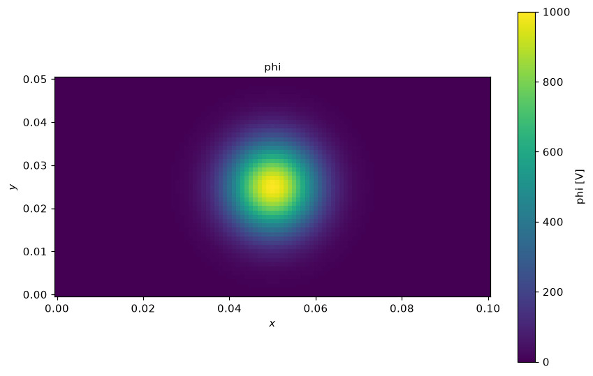
phi.plot(y=0.025, name="phi", units="V");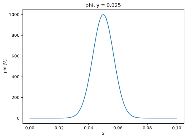
Computing with fields
Section titled “Computing with fields”Fields combine elementwise with numbers, arrays and other fields on the same grid; NumPy
ufuncs apply too. gradient differentiates a scalar field into a vector field with one
component per axis; a scalar field broadcasts over the components of a vector field, so
E / |E| is a unit vector field.
E = -phi.gradient()magnitude = E.magnitude()unit = E / (magnitude + 1e-12)print(E.num_components, magnitude.num_components, float(unit.magnitude().max()))magnitude.plot(name="|E|", units="V/m", equal_aspect=True);2 1 1.0000000000000002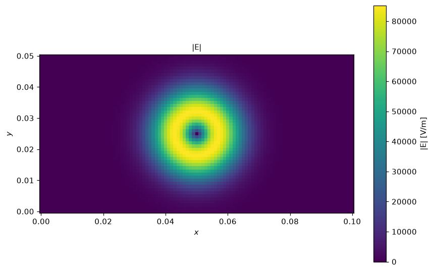
E.evaluate(name="E").plasma.plot.vector(x="x", y="y", stride=6);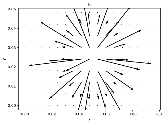
Saving
Section titled “Saving”export writes a NetCDF file with the values, the bounds and the periodic axes; load
reads it back, split over the ranks as asked.
import tempfilefrom pathlib import Path
path = Path(tempfile.mkdtemp()) / "phi.nc"phi.export(path)again = Field.load(path)print(again, np.array_equal(again.to_numpy(), phi.to_numpy()))
Field(ndim=2, num_gridpoints=(101, 51), num_components=1, lower_bound=(0.0, 0.0), upper_bound=(0.1, 0.05), distributed=False)rank 0: stored block (101, 51, 1), index bounds [(0, 101), (0, 51)] True