Prescribed electric field

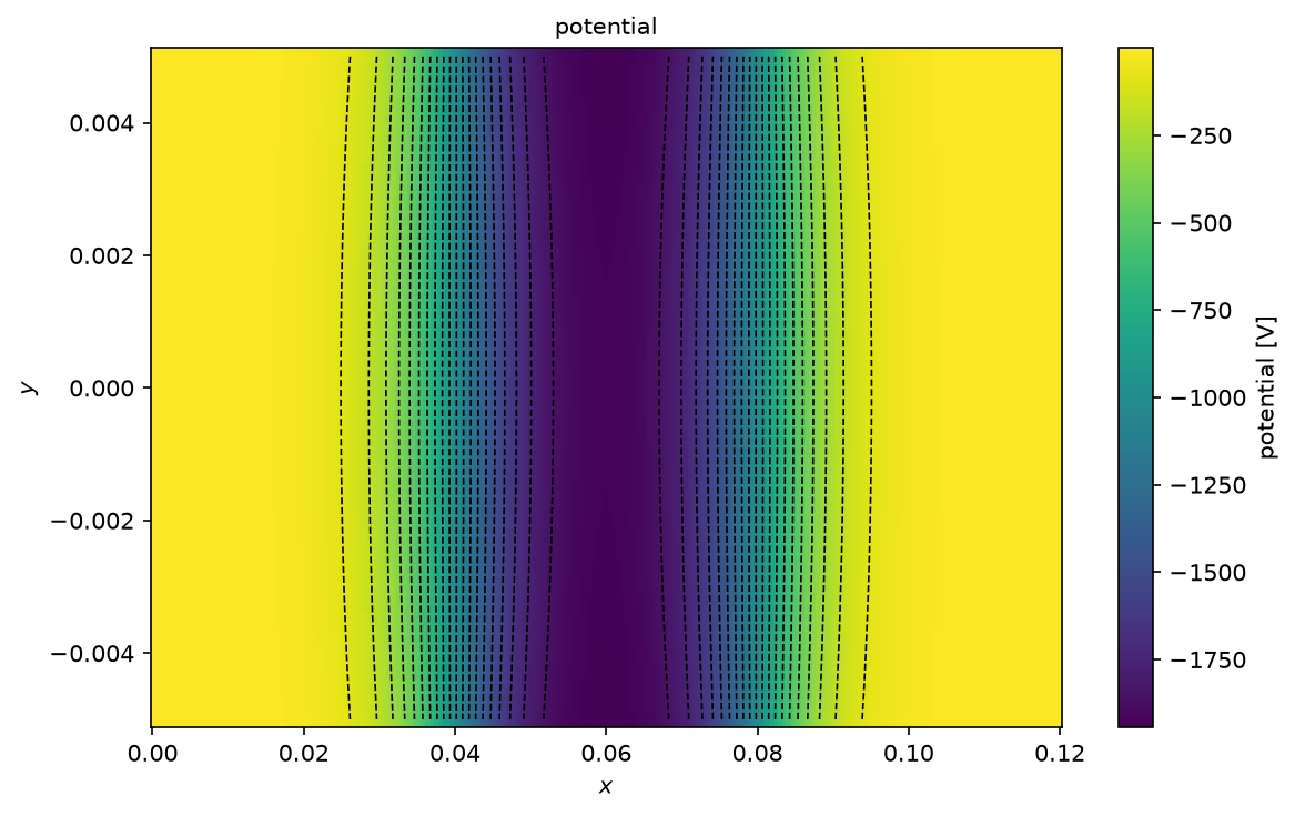
An electric field from a prescribed potential: build $E = -\nabla\phi$ on a grid from a potential given as a function, here a three-electrode lens.

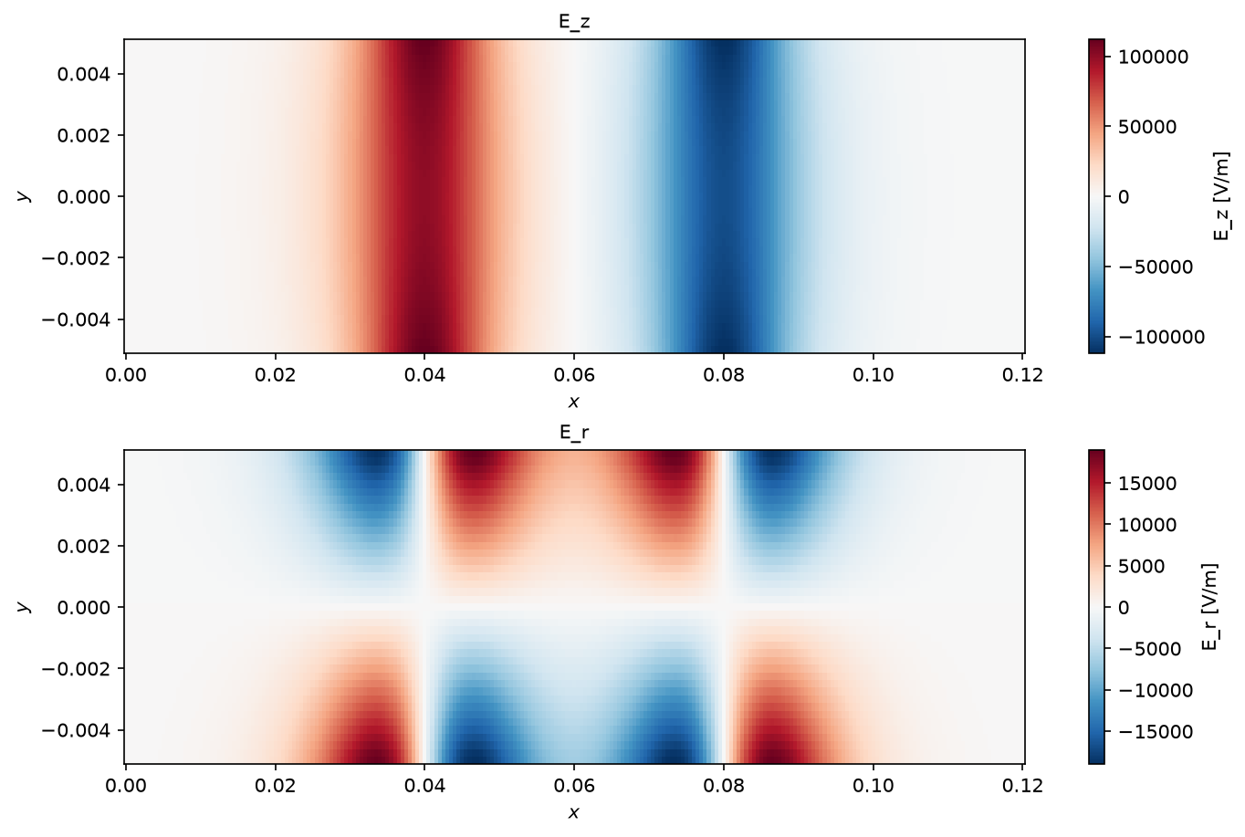
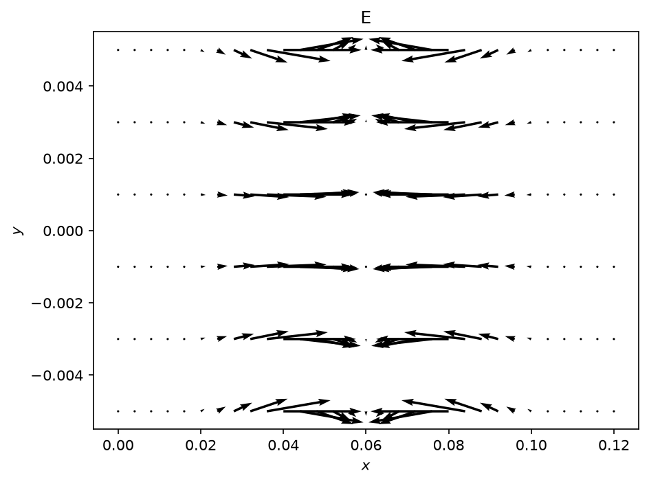
electric_field_from_potential evaluates the potential on the nodes and differentiates it with second-order central differences. The lens has three cylinders, the middle one at $-2$ kV, with smooth steps $\phi_0(z)$ between them; off the axis the potential is the paraxial expansion $\phi(z, r) = \phi_0(z) - \frac{r^2}{4}\phi_0''(z)$. The maps show the potential and both field components, the arrows the field. The radial field $E_r = \frac{r}{2}\phi_0''$ changes sign within each gap, so each gap focuses on one side and defocuses on the other; the net effect of such an einzel lens is focusing.

Python source

"""Prescribed electric field

An electric field from a prescribed potential: build $E = -\\nabla\\phi$ on a grid from a potential given as a function, here a three-electrode lens.

`electric_field_from_potential` evaluates the potential on the nodes and differentiates it
with second-order central differences. The lens has three cylinders, the middle one at
$-2$ kV, with smooth steps $\\phi_0(z)$ between them; off the axis the potential is the
paraxial expansion $\\phi(z, r) = \\phi_0(z) - \\frac{r^2}{4}\\phi_0''(z)$. The maps show the
potential and both field components, the arrows the field. The radial field
$E_r = \\frac{r}{2}\\phi_0''$ changes sign within each gap, so each gap focuses on one side
and defocuses on the other; the net effect of such an einzel lens is focusing.
"""

import matplotlib.pyplot as plt
import numpy as np
import plasma_plots  # noqa: F401

from mpifield import Field, electric_field_from_potential

voltage, width = -2000.0, 0.01  # the middle electrode, the step width (m)
gaps = (0.04, 0.08)  # the centres of the two gaps (m)


def axial(z):
    """phi_0 and phi_0'' on the axis: two tanh steps."""
    up, down = (np.tanh((z - gap) / width) for gap in gaps)
    phi = 0.5 * voltage * (up - down)
    second = -voltage / width**2 * (up * (1 - up**2) - down * (1 - down**2))
    return phi, second


def potential(z, r):
    """The paraxial potential of the lens (V) at ``z`` and ``r`` (m)."""
    phi, second = axial(z)
    return phi - r**2 / 4 * second


kwargs = {"lower_bound": (0.0, -0.005), "upper_bound": (0.12, 0.005)}
field = electric_field_from_potential(potential, num_gridpoints=(241, 41), **kwargs)
nodes = np.meshgrid(*field.get_grid_points(), indexing="ij")
phi = Field.from_array(potential(*nodes), **kwargs)

phi.plot(name="potential", units="V", levels=20)
fig, axes = plt.subplots(2, 1, figsize=(9, 6), layout="constrained")
field.plot(
    ax=axes[0], component=0, name="E_z", units="V/m", cmap="RdBu_r", symmetric=True
)
field.plot(
    ax=axes[1], component=1, name="E_r", units="V/m", cmap="RdBu_r", symmetric=True
)
arrows = field.evaluate(name="E", units="V/m")
arrows.plasma.plot.vector(x="x", y="y", stride=8)
plt.show()

Plots