Test particles

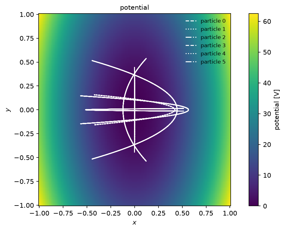
Test particles in a fixed field: push charged particles through a field on a grid with a leapfrog scheme, gathering the field every step.

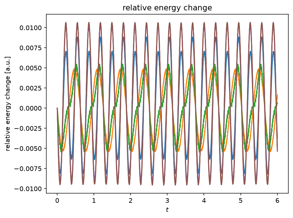
This is the loop of a test-particle code: gather gives the electric field at all markers at once, from the compiled gather. The field is that of a 2D potential well, $\phi = \phi_0 (x^2 + y^2/4)$, so the orbits are Lissajous figures with frequencies in the ratio 2:1, and the energy is conserved to the accuracy of the scheme.

Python source

"""Test particles

Test particles in a fixed field: push charged particles through a field on a grid with a leapfrog scheme, gathering the field every step.

This is the loop of a test-particle code: `gather` gives the electric field at
all markers at once, from the compiled gather. The field is that of a 2D potential well,
$\\phi = \\phi_0 (x^2 + y^2/4)$, so the orbits are Lissajous figures with frequencies in the
ratio 2:1, and the energy is conserved to the accuracy of the scheme.
"""

import matplotlib.pyplot as plt
import numpy as np
import plasma_plots  # noqa: F401
import xarray as xr

from mpifield import Field

kwargs = {"ndim": 2, "lower_bound": (-1.0, -1.0), "upper_bound": (1.0, 1.0)}
phi = Field(num_gridpoints=129, **kwargs)
x, y = np.meshgrid(*phi.get_grid_points(), indexing="ij")
phi.set_field_data(50.0 * (x**2 + y**2 / 4))
electric = -phi.gradient()

charge_over_mass = 1.0  # a positive charge in a potential well
rng = np.random.default_rng(11)
positions = rng.uniform(-0.6, 0.6, (2, 6))
velocities = np.zeros_like(positions)
dt, steps = 2e-3, 3000
paths = [positions.copy()]
energy = []
for _ in range(steps):
    velocities += charge_over_mass * electric.gather(positions) * dt
    positions += velocities * dt
    paths.append(positions.copy())
    kinetic = 0.5 * (velocities**2).sum(axis=0)
    energy.append(kinetic + charge_over_mass * phi.gather(positions)[0])
paths = np.array(paths)
energy = np.array(energy)

lines = {
    f"particle {i}": (paths[:, 0, i], paths[:, 1, i]) for i in range(paths.shape[2])
}
phi.plot(name="potential", units="V", overlays={"lines": lines}, equal_aspect=True)
drift = xr.DataArray(
    (energy - energy[0]) / np.abs(energy[0]),
    dims=("t", "particle"),
    coords={"t": dt * np.arange(1, steps + 1)},
    name="relative energy change",
)
result = drift.plasma.plot.lineout(x="t", particle=0)
for i in range(1, paths.shape[2]):
    drift.plasma.plot.lineout(x="t", particle=i, ax=result.ax)
plt.show()

Plots