Gather and scatter

Download notebook View on GitHubRun when the site was built.

Deposit marker values onto the nodes and interpolate the field at the markers, with linear, quadratic or your own weights.

These are the two grid operations of every particle-in-cell code. Both use the same (cloud-in-cell) weights: a marker in a cell shares its value among the cell’s corners in proportion to the opposite sub-volumes, and reads the field back from them with the same weights. Positions are component-major, (ndim, N), values (ncomp, N).

import numpy as np
import plasma_plots  # noqa: F401
import xarray as xr

from mpifield import QUADRATIC, Field, Weighting

rng = np.random.default_rng(0)

One marker

A marker a quarter of the way through a 1D cell gives three quarters of its value to the left node and one quarter to the right one.

line = Field(ndim=1, lower_bound=(0.0,), upper_bound=(1.0,), num_gridpoints=5)
line.scatter(np.array([[0.3125]]), 1.0)  # 1.25 cells from the first node
print(line.local[:, 0])

[0.   0.75 0.25 0.   0.  ]

A density from markers

scatter adds to what is on the grid, so the field is zeroed between steps (set_field_data(0.0)). The deposit conserves the total exactly; divided by the cell area it is a density.

count = 50_000
positions = np.stack([rng.normal(0.5, 0.12, count), rng.normal(0.5, 0.06, count)])
weights = np.full((1, count), 1e12 / count)  # 1e12 physical particles in all

density = Field(
    ndim=2, lower_bound=(0.0, 0.0), upper_bound=(1.0, 1.0), num_gridpoints=65
)
density.scatter(positions, weights)
print(f"deposited {density.sum():.6e} of {weights.sum():.6e}")
area = float(np.prod(density.grid_spacing))
(density / area).plot(name="density", units="1/m^2", equal_aspect=True);

deposited 1.000000e+12 of 1.000000e+12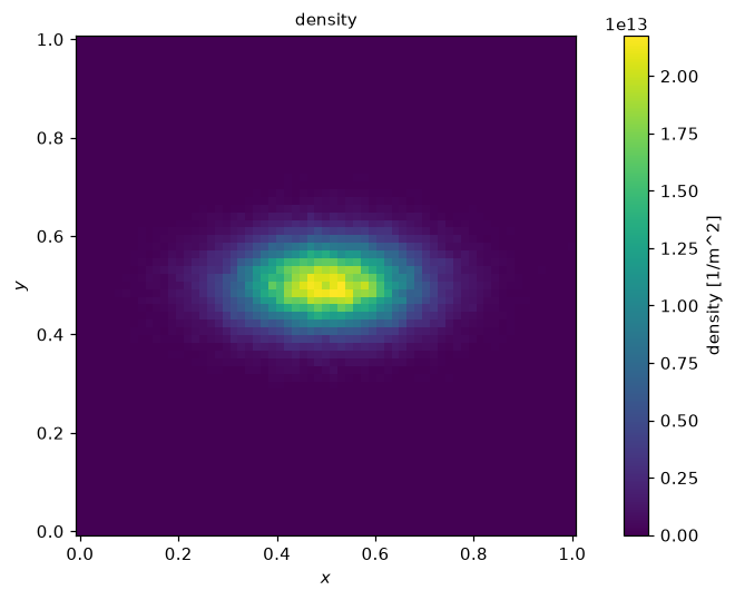

Gathering the field at the markers

gather returns (num_components, N): here the two components of the field of a potential with a known gradient, so the gathered field can be checked. Linear interpolation reproduces a linear field exactly and is second-order accurate otherwise.

phi = Field(ndim=2, lower_bound=(0.0, 0.0), upper_bound=(1.0, 1.0), num_gridpoints=65)
x, y = np.meshgrid(*phi.get_grid_points(), indexing="ij")
phi.set_field_data(np.sin(np.pi * x) * np.sin(np.pi * y))
E = -phi.gradient()

gathered = E.gather(positions)  # (2, N)
exact_x = -np.pi * np.cos(np.pi * positions[0]) * np.sin(np.pi * positions[1])
print(gathered.shape, "largest error in E_x:", np.abs(gathered[0] - exact_x).max())

(2, 50000) largest error in E_x: 0.06738897529658106

Deposit and gather are transposes

With the same weights, $\sum_i q_i\, g(x_i) = \sum_n g_n \rho_n$ for any field $g$ and the deposit $\rho$ of the charges $q_i$ . In a PIC code this means momentum conservation and no self-force on a uniform grid.

g = phi
rho = Field(ndim=2, lower_bound=(0.0, 0.0), upper_bound=(1.0, 1.0), num_gridpoints=65)
charges = rng.normal(size=count)
rho.scatter(positions, charges)
print(float(g.gather(positions)[0] @ charges), float((g * rho).sum()))

-40.32960873796823 -40.32960873796801

Other weightings

scatter and gather take a Weighting, linear (LINEAR) by default. QUADRATIC is the quadratic B-spline: a marker shares its value among its nearest node and the two around it, in each axis, with weights $(1/2 - d)^2/2$ , $3/4 - d^2$ and $(1/2 + d)^2/2$ for its offset $d$ from the nearest node. It is smoother (less grid noise, a continuous force) for $3^{d}$ nodes per marker instead of $2^{d}$ , and needs two halo nodes on a split field instead of one. A weighting holds both kernels, so the deposit and the gather stay transposes of each other.

line = Field(ndim=1, lower_bound=(0.0,), upper_bound=(1.0,), num_gridpoints=5)
line.scatter(np.array([[0.5]]), 1.0, QUADRATIC)  # on node 2
print(line.local[:, 0])

rho = Field(ndim=2, lower_bound=(0.0, 0.0), upper_bound=(1.0, 1.0), num_gridpoints=65)
rho.scatter(positions, charges, QUADRATIC)
print(float(g.gather(positions, QUADRATIC)[0] @ charges), float((g * rho).sum()))

[0.    0.125 0.75  0.125 0.   ]
-40.34179200676893 -40.341792006768245

A weighting of your own is a scatter and a gather function (or compiled kernel) for each number of dimensions it covers, with the arguments of the kernel convention in mpifield.weighting: the markers (ndim, N), their values or the result (ncomp, N), the grid num_nodes + (ncomp,), then the lower corner, the node spacing, the node counts and the periodic flags, one per axis each. Here the nearest grid point, in NumPy, for 2D fields only:

def nearest_nodes(positions, lower, cell, num):
    return tuple(
        np.clip(np.rint((positions[d] - lower[d]) / cell[d]).astype(int), 0, num[d] - 1)
        for d in range(len(num))
    )


def scatter_nearest(positions, values, field, *geometry):
    nodes = nearest_nodes(positions, geometry[0:2], geometry[2:4], geometry[4:6])
    np.add.at(field, nodes, values.T)


def gather_nearest(positions, field, result, *geometry):
    nodes = nearest_nodes(positions, geometry[0:2], geometry[2:4], geometry[4:6])
    result[...] = field[nodes].T


NEAREST = Weighting(
    "nearest", scatter={2: scatter_nearest}, gather={2: gather_nearest}, halo=1
)
rho = Field(ndim=2, lower_bound=(0.0, 0.0), upper_bound=(1.0, 1.0), num_gridpoints=65)
rho.scatter(positions, charges, NEAREST)
print(float(g.gather(positions, NEAREST)[0] @ charges), float((g * rho).sum()))

-39.83529101757544 -39.835291017575756

Periodic axes and the edges

On a periodic axis the last node neighbours the first; markers in the last cell deposit onto both, and positions beyond the period wrap. On a bounded axis a marker outside the grid uses the edge cell with its weight clamped to [0, 1], so it gets the edge value.

ring = Field(
    ndim=1, lower_bound=(0.0,), upper_bound=(1.0,), num_gridpoints=4, periodic=True
)
ring.scatter(np.array([[0.875, 1.875]]), 1.0)  # mid-way between nodes 3 and 0, twice
print("periodic:", ring.local[:, 0])

edge = Field(ndim=1, lower_bound=(0.0,), upper_bound=(1.0,), num_gridpoints=5)
edge.set_field_data(np.arange(5.0))
print("bounded, outside:", edge.gather(np.array([[-0.5, 1.5]])))

periodic: [1. 0. 0. 1.]
bounded, outside: [[0. 4.]]

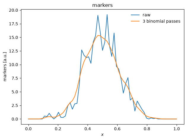
Smoothing

Deposits with few markers per cell are noisy. smooth applies a short separable filter along each axis, as PIC codes do before the field solve; the binomial filter removes the grid-scale noise and keeps the total.

few = Field(ndim=2, lower_bound=(0.0, 0.0), upper_bound=(1.0, 1.0), num_gridpoints=65)
few.scatter(positions[:, :3000], np.ones((1, 3000)))
smoothed = few.smooth_binomial(passes=3, in_place=False)
profiles = xr.concat(
    [few.evaluate(y=0.5, name="markers"), smoothed.evaluate(y=0.5, name="markers")],
    dim=xr.DataArray(["raw", "smoothed"], dims="deposit"),
)
result = profiles.isel(deposit=0).plasma.plot.lineout(x="x")
profiles.isel(deposit=1).plasma.plot.lineout(x="x", ax=result.ax)
result.ax.legend(["raw", "3 binomial passes"], frameon=False);