Smoothing filters

The binomial, Gaussian and uniform filters of Field.smooth, as low-pass filters of a noisy deposit.

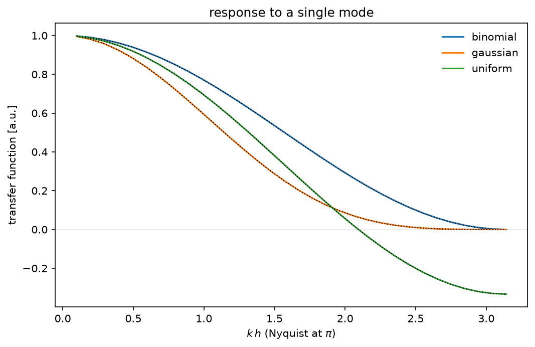
Each filter is a short symmetric stencil applied along each axis; its transfer function is the cosine series of the stencil. The binomial $[1,2,1]/4$ removes the grid-scale (Nyquist) mode completely, the 5-point Gaussian $[1,4,6,4,1]/16$ is that filter twice, and the 3-point average $[1,1,1]/3$ keeps a third of the Nyquist mode with the opposite sign. The plot measures the response of each filter to single Fourier modes on a periodic grid and compares it with the formula.

Python source

"""Smoothing filters

The binomial, Gaussian and uniform filters of `Field.smooth`, as low-pass filters of a noisy deposit.

Each filter is a short symmetric stencil applied along each axis; its transfer function is
the cosine series of the stencil. The binomial $[1,2,1]/4$ removes the grid-scale (Nyquist)
mode completely, the 5-point Gaussian $[1,4,6,4,1]/16$ is that filter twice, and the 3-point
average $[1,1,1]/3$ keeps a third of the Nyquist mode with the opposite sign. The plot
measures the response of each filter to single Fourier modes on a periodic grid and compares
it with the formula.
"""

import matplotlib.pyplot as plt
import numpy as np
import plasma_plots  # noqa: F401
import xarray as xr

from mpifield import Field

n = 64
kwargs = {"ndim": 1, "lower_bound": (0.0,), "upper_bound": (1.0,), "periodic": True}
modes = np.arange(1, n // 2 + 1)
theta = 2 * np.pi * modes / n
formulas = {
    "binomial": np.cos(theta / 2) ** 2,
    "gaussian": np.cos(theta / 2) ** 4,
    "uniform": (1 + 2 * np.cos(theta)) / 3,
}
fig, ax = plt.subplots(figsize=(7, 4.5), layout="constrained")
for name, formula in formulas.items():
    response = []
    for k in modes:
        field = Field(num_gridpoints=n, **kwargs)
        (x,) = field.get_grid_points()
        field.set_field_data(np.cos(2 * np.pi * k * x))
        filtered = field.smooth(filter_name=name, in_place=False)
        response.append(float(filtered.local[0, 0]))  # the cosine's peak at x = 0
    measured = xr.DataArray(
        response, dims="kh", coords={"kh": theta}, name="transfer function"
    )
    measured.plasma.plot.lineout(x="kh", ax=ax)
    ax.lines[-1].set_label(name)
    ax.plot(theta, formula, "k:", lw=1)
ax.axhline(0, color="0.6", lw=0.5)
ax.set(xlabel=r"$k\,h$ (Nyquist at $\pi$)", title="response to a single mode")
ax.legend(frameon=False)
plt.show()

Plots