E x B drift

Vector fields: combine fields with arithmetic, gradient, cross, dot and magnitude: the drift velocity of a magnetized plasma.

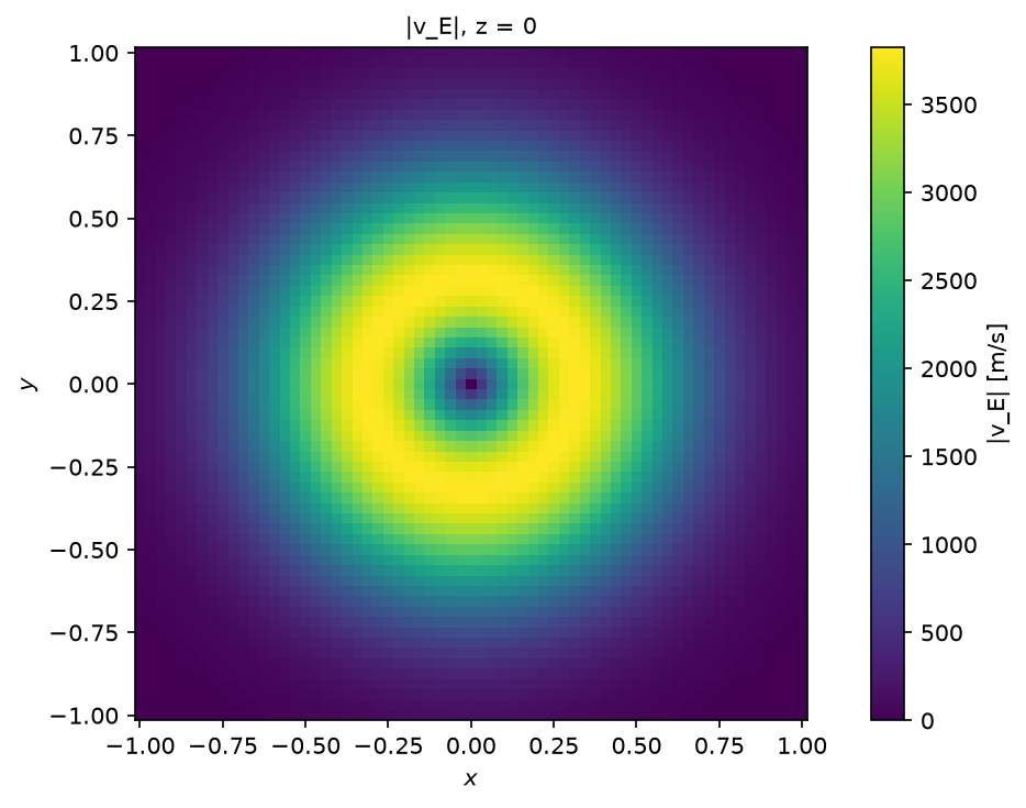
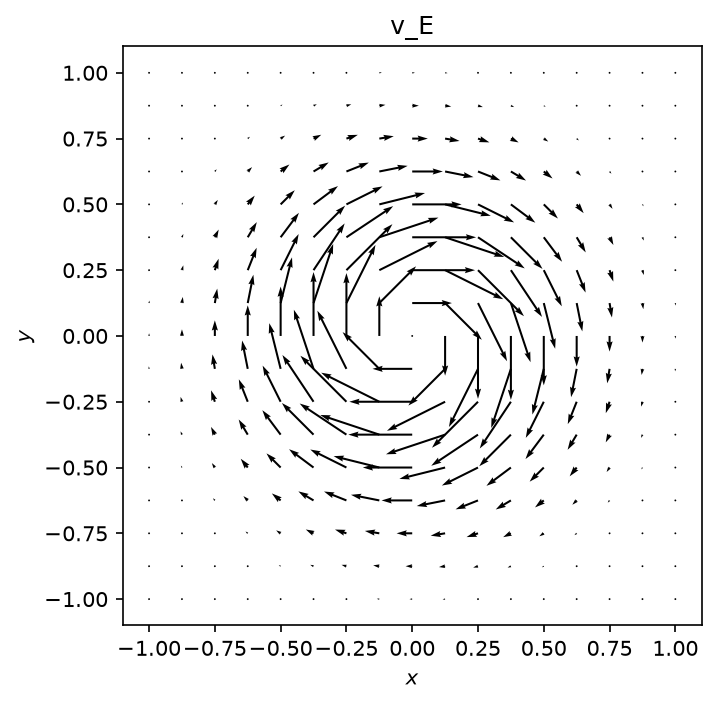
A potential hill $\phi = \phi_0 e^{-r^2/w^2}$ in a uniform magnetic field $B \hat z$ makes the guiding centres drift with $v_E = E \times B / B^2$, along the equipotentials. The drift is a field computed from fields: the gradient of the potential, a cross product with a constant field and a division by $B^2$ from dot. Its divergence-free circulation shows as closed loops; its speed peaks where the field is strongest.

Python source

"""E x B drift

Vector fields: combine fields with arithmetic, `gradient`, `cross`, `dot` and `magnitude`: the drift velocity of a magnetized plasma.

A potential hill $\\phi = \\phi_0 e^{-r^2/w^2}$ in a uniform magnetic field $B \\hat z$ makes
the guiding centres drift with $v_E = E \\times B / B^2$, along the equipotentials. The
drift is a field computed from fields: the gradient of the potential, a cross product with a
constant field and a division by $B^2$ from `dot`. Its divergence-free circulation shows as
closed loops; its speed peaks where the field is strongest.
"""

import matplotlib.pyplot as plt
import numpy as np
import plasma_plots  # noqa: F401

from mpifield import Field

kwargs = {"ndim": 3, "lower_bound": (-1.0, -1.0, -0.1), "upper_bound": (1.0, 1.0, 0.1)}
shape = (65, 65, 3)
phi = Field(num_gridpoints=shape, **kwargs)
x, y, _ = np.meshgrid(*phi.get_grid_points(), indexing="ij")
phi.set_field_data(100.0 * np.exp(-(x**2 + y**2) / 0.2))

electric = -phi.gradient()
magnetic = Field(num_gridpoints=shape, num_components=3, **kwargs)
magnetic.set_field_data(0.05, component=2)  # 50 mT along z
drift = electric.cross(magnetic) / magnetic.dot(magnetic)
speed = drift.magnitude()
print(f"largest drift speed {speed.max():.0f} m/s")

speed.plot(z=0.0, name="|v_E|", units="m/s", equal_aspect=True)
arrows = drift.evaluate(z=0.0, name="v_E")
result = arrows.sel(component=[0, 1]).plasma.plot.vector(x="x", y="y", stride=4)
result.ax.set_aspect("equal")
plt.show()

Plots