Tutorial 13 – Advanced Matplotlib Plotting
Advanced Matplotlib plotting
This tutorial covers horizontal bars, histograms, filled regions, reference spans, arrows, infinitely extending lines, and secondary y-axes.
[1]:
import numpy as np
from maxplotlib import Canvas

x = np.linspace(0, 2 * np.pi, 200)
Common plotting primitives
[2]:
canvas = Canvas(width="12cm", ratio=0.65)
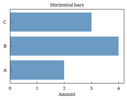
canvas.barh([0, 1, 2], [2, 4, 3], color="steelblue", alpha=0.8)
canvas.set_yticks([0, 1, 2], labels=["A", "B", "C"])
canvas.set_xlabel("Amount")
canvas.set_title("Horizontal bars")
canvas.show()
[2]:
(<Figure size 472.441x307.087 with 1 Axes>,
 array([[<Axes: title={'center': 'Horizontal bars'}, xlabel='Amount'>]],
       dtype=object))
[3]:
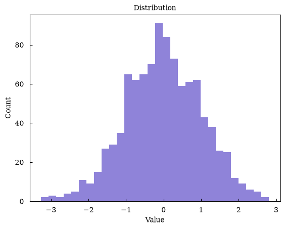
samples = np.random.default_rng(4).normal(size=1000)
canvas = Canvas()
canvas.hist(samples, bins=30, color="slateblue", alpha=0.75)
canvas.set_xlabel("Value")
canvas.set_ylabel("Count")
canvas.set_title("Distribution")
canvas.show()
[3]:
(<Figure size 640x480 with 1 Axes>,
 array([[<Axes: title={'center': 'Distribution'}, xlabel='Value', ylabel='Count'>]],
       dtype=object))
Steps, stairs, broken bars, and pie charts
[4]:
canvas = Canvas()
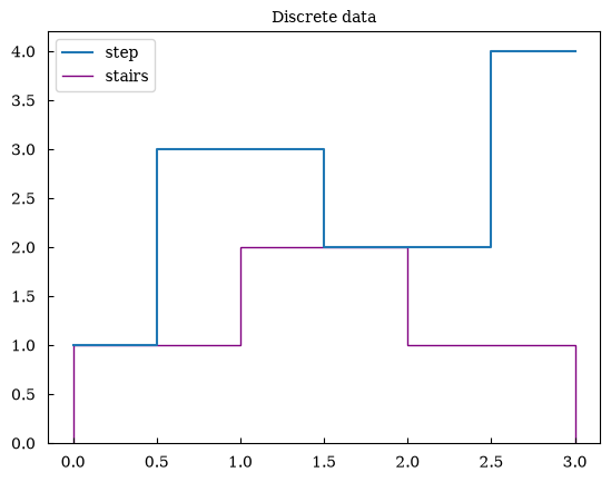
canvas.step([0, 1, 2, 3], [1, 3, 2, 4], where="mid", label="step")
canvas.stairs([1, 2, 1], edges=[0, 1, 2, 3], color="purple", label="stairs")
canvas.set_title("Discrete data")
canvas.set_legend(True)
canvas.show()
[4]:
(<Figure size 640x480 with 1 Axes>,
 array([[<Axes: title={'center': 'Discrete data'}>]], dtype=object))
[5]:
canvas = Canvas()
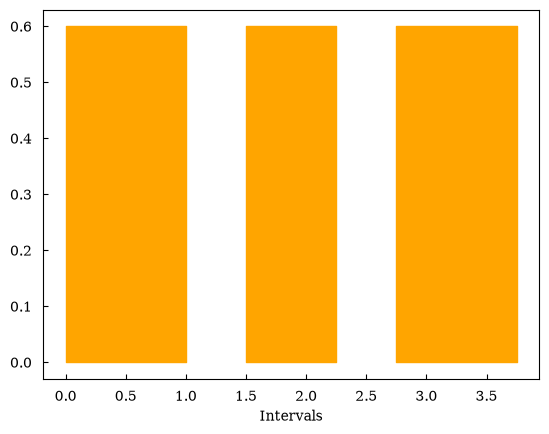
canvas.broken_barh([(0, 1), (1.5, 0.75), (2.75, 1.0)], (0, 0.6), color="orange")
canvas.set_xlabel("Intervals")
canvas.show()
[5]:
(<Figure size 640x480 with 1 Axes>,
 array([[<Axes: xlabel='Intervals'>]], dtype=object))
[6]:
canvas = Canvas()
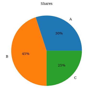
canvas.pie([30, 45, 25], labels=["A", "B", "C"], autopct="%1.0f%%")
canvas.set_title("Shares")
canvas.show()
[6]:
(<Figure size 640x480 with 1 Axes>,
 array([[<Axes: title={'center': 'Shares'}>]], dtype=object))
Regions, arrows, and reference lines
[7]:
canvas = Canvas()
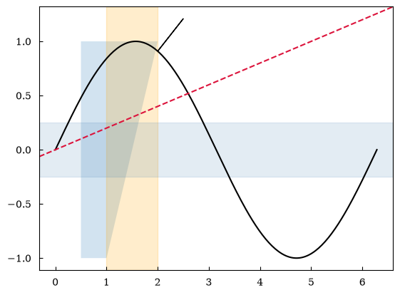
canvas.plot(x, np.sin(x), color="black")
canvas.fill_betweenx([-1, 0, 1], 0.5, [1.0, 1.5, 2.0], alpha=0.2)
canvas.axvspan(1.0, 2.0, color="orange", alpha=0.2)
canvas.axhspan(-0.25, 0.25, color="steelblue", alpha=0.15)
canvas.arrow(2.0, np.sin(2.0), 0.5, 0.3, length_includes_head=True)
canvas.axline((0, 0), slope=0.2, linestyle="--", color="crimson")
canvas.show()
[7]:
(<Figure size 640x480 with 1 Axes>, array([[<Axes: >]], dtype=object))
Secondary y-axis
[8]:
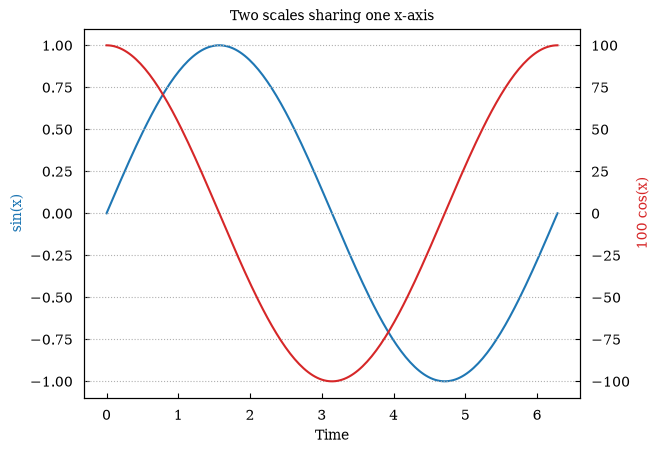
twin_canvas, primary = Canvas.subplots()
secondary = twin_canvas.twinx()

primary.plot(x, np.sin(x), color="tab:blue")
secondary.plot(x, 100 * np.cos(x), color="tab:red")
primary.set_xlabel("Time")
primary.set_ylabel("sin(x)", color="tab:blue")
secondary.set_ylabel("100 cos(x)", color="tab:red")
twin_canvas.set_title("Two scales sharing one x-axis")
twin_canvas.show()
[8]:
(<Figure size 640x480 with 2 Axes>,
 array([[<Axes: title={'center': 'Two scales sharing one x-axis'}, xlabel='Time', ylabel='sin(x)'>]],
       dtype=object))
Secondary y-axes are supported by the Matplotlib and Plotly backends. The plotext and TikZ backends currently reject a canvas containing twinx() plots instead of silently producing an incorrect figure.
Scientific field plots
[9]:
x = np.linspace(-1, 1, 40)
y = np.linspace(-1, 1, 40)
xx, yy = np.meshgrid(x, y)
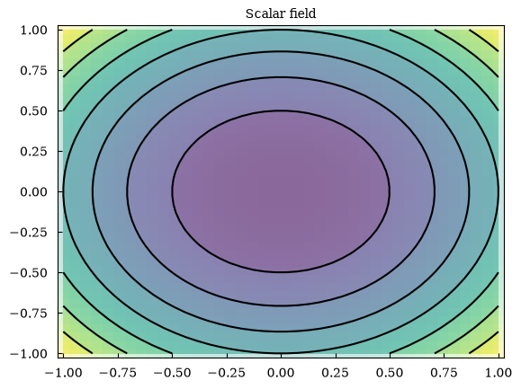
z = xx**2 + yy**2

canvas = Canvas()
canvas.contour(x, y, z, colors="black")
canvas.contourf(x, y, z, alpha=0.5)
canvas.pcolormesh(x, y, z, alpha=0.25)
canvas.set_title("Scalar field")
canvas.show()
[9]:
(<Figure size 640x480 with 1 Axes>,
 array([[<Axes: title={'center': 'Scalar field'}>]], dtype=object))
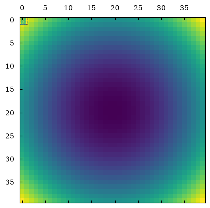
For point-density data and matrix-oriented displays:
[10]:
canvas = Canvas()
canvas.hexbin(xx.ravel(), yy.ravel(), gridsize=12)
canvas.matshow(z)
canvas.show()
[10]:
(<Figure size 640x480 with 1 Axes>, array([[<Axes: >]], dtype=object))
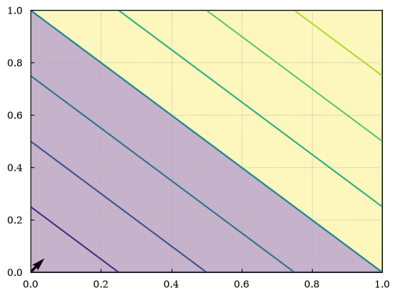
Unstructured triangular data and vector fields are also supported:
[11]:
points_x = np.array([0.0, 1.0, 0.0, 1.0])
points_y = np.array([0.0, 0.0, 1.0, 1.0])
triangles = [[0, 1, 2], [1, 3, 2]]
values = points_x + points_y

canvas = Canvas()
canvas.quiver(points_x, points_y, np.ones(4), np.ones(4))
canvas.triplot(points_x, points_y, triangles=triangles)
canvas.tripcolor(points_x, points_y, values, triangles=triangles, alpha=0.3)
canvas.tricontour(points_x, points_y, values, triangles=triangles)
canvas.show()
[11]:
(<Figure size 640x480 with 1 Axes>, array([[<Axes: >]], dtype=object))
Statistical and event plots
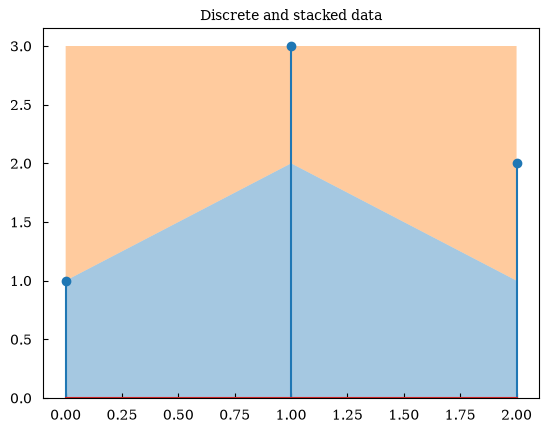
[12]:
canvas = Canvas()
canvas.stem([0, 1, 2], [1, 3, 2])
canvas.stackplot([0, 1, 2], [1, 2, 1], [2, 1, 2], alpha=0.4)
canvas.set_title("Discrete and stacked data")
canvas.show()
[12]:
(<Figure size 640x480 with 1 Axes>,
 array([[<Axes: title={'center': 'Discrete and stacked data'}>]],
       dtype=object))
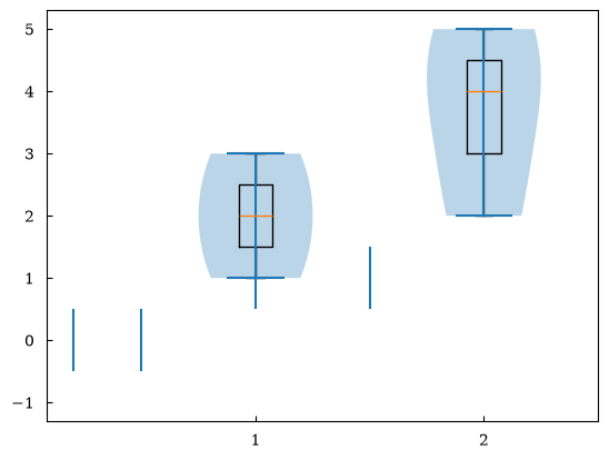
[13]:
canvas = Canvas()
canvas.boxplot([[1, 2, 3], [2, 4, 5]])
canvas.violinplot([[1, 2, 3], [2, 4, 5]])
canvas.eventplot([[0.2, 0.5], [1.0, 1.5]])
canvas.show()
[13]:
(<Figure size 640x480 with 1 Axes>, array([[<Axes: >]], dtype=object))