Tutorial 06 – Layers
Layers let you assign each piece of data to a numbered layer. You can then render a subset of layers — e.g. to reveal a derivation step by step, or to produce separate PDF overlays from a single source file.
[1]:
from maxplotlib import Canvas
import numpy as np
Backend selection
All examples in this tutorial use the same Canvas API; you can switch rendering backends at any time:
BACKEND = "matplotlib"for static Matplotlib outputBACKEND = "plotly"for interactive Plotly output (Jupyter-friendly)
Most cells end with canvas.show(backend=BACKEND) so you can re-run the whole notebook with a different backend.
[2]:
# Change to "plotly" for interactive output
BACKEND = "matplotlib"
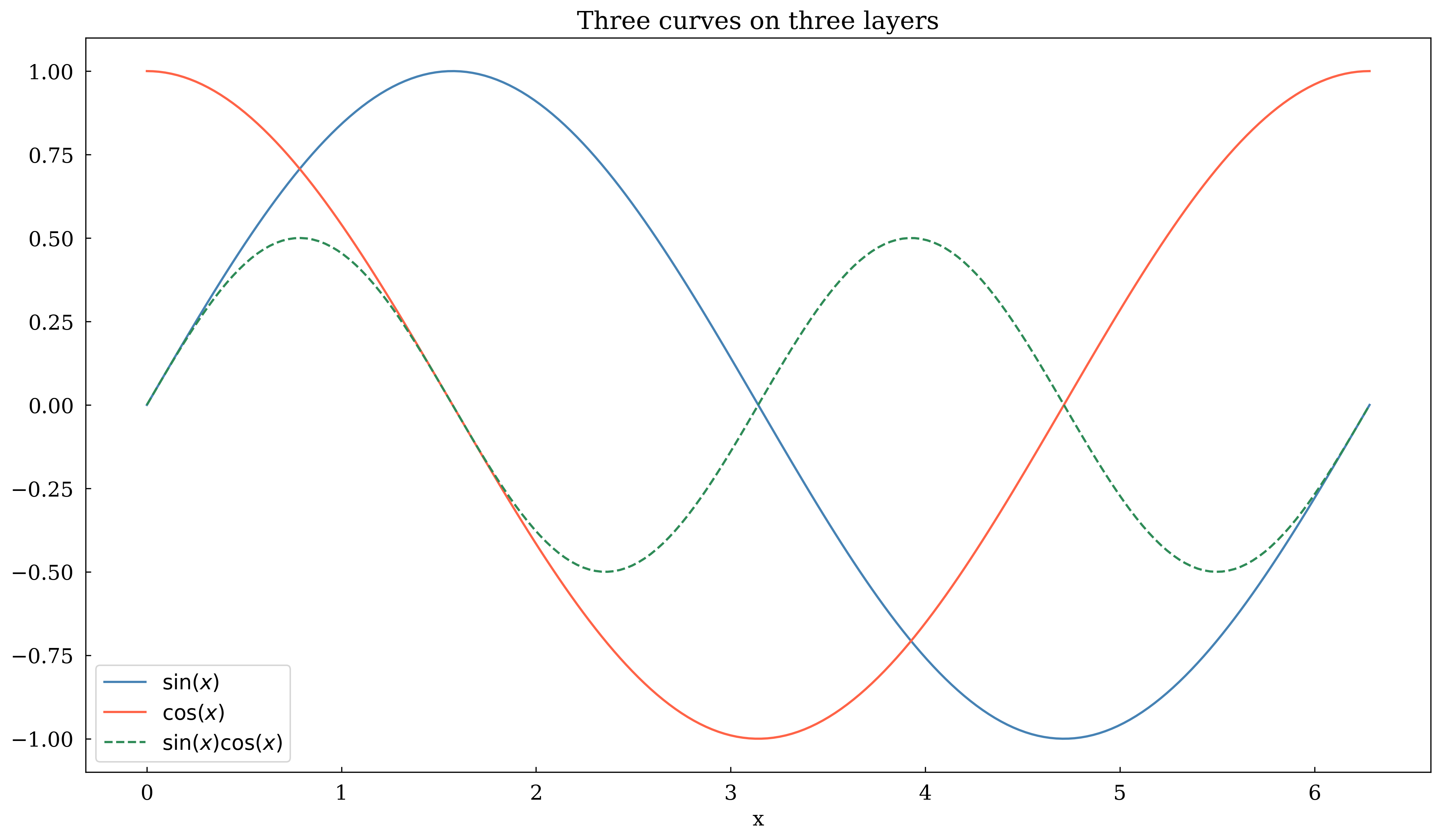
1 · Assigning data to layers
Pass layer=<int> to any plot call. Layers are just integer tags — the default is 0.
[3]:
x = np.linspace(0, 2 * np.pi, 200)

canvas, ax = Canvas.subplots(width="10cm", ratio=0.55)

ax.plot(x, np.sin(x), color="steelblue", label=r"$\sin(x)$", layer=0)
ax.plot(x, np.cos(x), color="tomato", label=r"$\cos(x)$", layer=1)
ax.plot(
    x,
    np.sin(x) * np.cos(x),
    color="seagreen",
    label=r"$\sin(x)\cos(x)$",
    linestyle="dashed",
    layer=2,
)

ax.set_xlabel("x")
ax.set_legend(True)
ax.set_title("Three curves on three layers")
canvas.show(backend=BACKEND)  # renders all layers by default
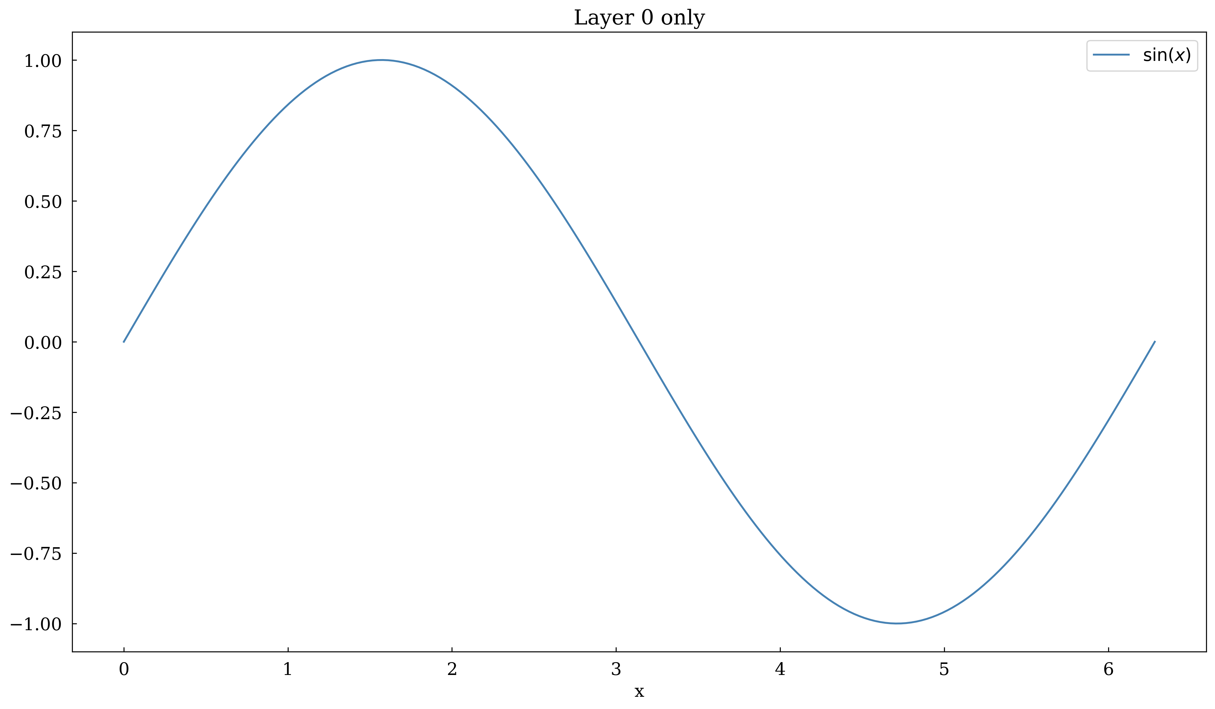
2 · Rendering specific layers
Pass layers=[...] to canvas.show() or canvas.savefig() to render only a subset of layers.
[4]:
x = np.linspace(0, 2 * np.pi, 200)

canvas, ax = Canvas.subplots(width="10cm", ratio=0.55)

ax.plot(x, np.sin(x), color="steelblue", label=r"$\sin(x)$", layer=0)
ax.plot(x, np.cos(x), color="tomato", label=r"$\cos(x)$", layer=1)
ax.plot(
    x,
    np.sin(x) * np.cos(x),
    color="seagreen",
    label=r"$\sin(x)\cos(x)$",
    linestyle="dashed",
    layer=2,
)

ax.set_xlabel("x")
ax.set_legend(True)

print("--- Layer 0 only ---")
ax.set_title("Layer 0 only")

canvas.show(backend=BACKEND, layers=[0])
--- Layer 0 only ---
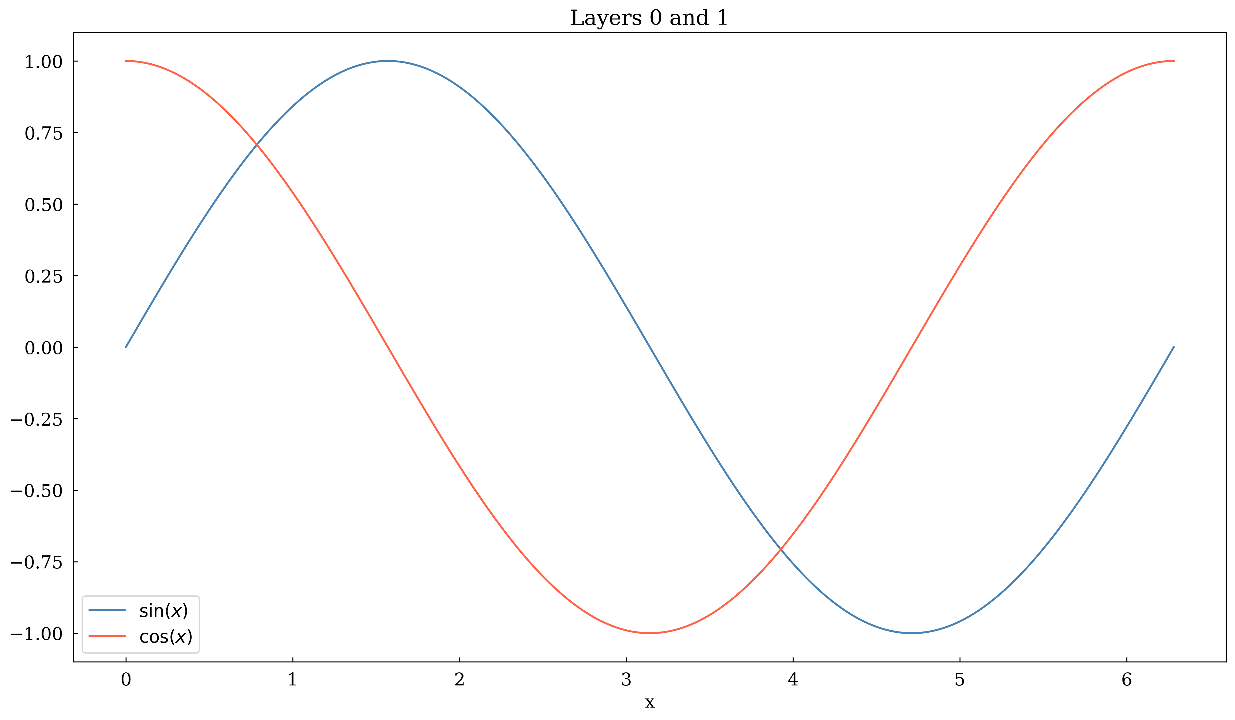
[5]:
# Same canvas — now show layers 0 and 1 together
ax.set_title("Layers 0 and 1")

canvas.show(backend=BACKEND, layers=[0, 1])
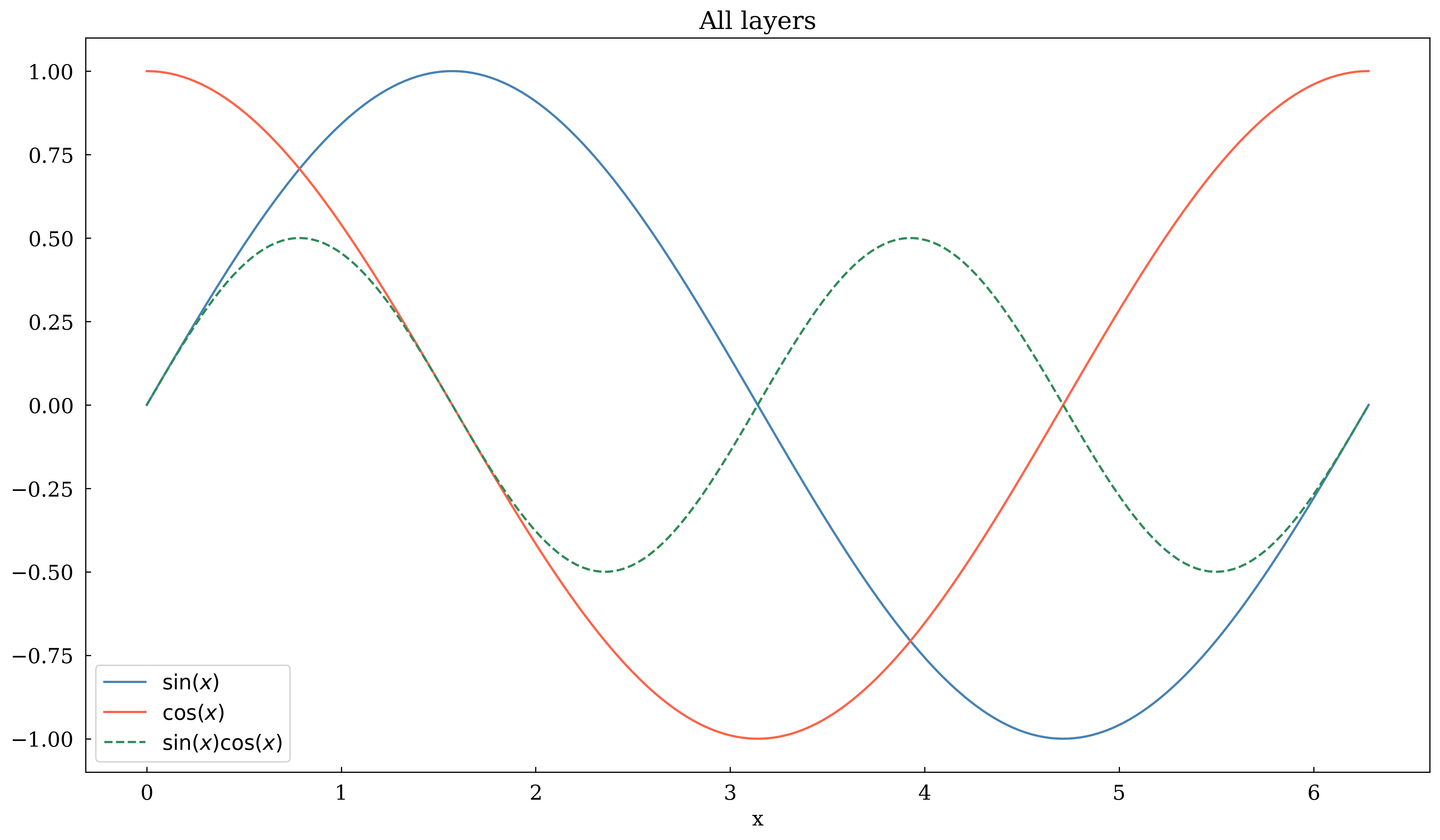
[6]:
# All layers
ax.set_title("All layers")

canvas.show(backend=BACKEND, layers=[0, 1, 2])
3 · Saving layer-by-layer
savefig with layer_by_layer=True writes one file per layer (e.g. fig_layer0.pdf, fig_layer1.pdf, …). This is ideal for building slide animations or LaTeX overlays.
[7]:
# Demonstration — not executed to avoid writing files during tutorial
#
# canvas.savefig('fig.pdf', layer_by_layer=True)
#
# Produces:
#   fig_layer0.pdf  (layer 0 only)
#   fig_layer1.pdf  (layers 0–1)
#   fig_layer2.pdf  (layers 0–2, i.e. all)
#
# Each file is a cumulative reveal, suitable for \includegraphics[<1->]{fig_layer0}
# in Beamer.
4 · Use case: progressively revealing a derivation
Build a plot where each layer adds the next step of a mathematical derivation.
[8]:
x = np.linspace(0, 2 * np.pi, 300)

canvas, ax = Canvas.subplots(width="11cm", ratio=0.6)

# Layer 0: raw data (noisy sine)
rng = np.random.default_rng(42)
y_data = np.sin(x) + rng.normal(0, 0.15, len(x))
ax.scatter(x, y_data, color="gray", s=8, alpha=0.5, label="measured data", layer=0)

# Layer 1: true function
ax.plot(x, np.sin(x), color="steelblue", linewidth=2, label=r"true: $\sin(x)$", layer=1)

# Layer 2: envelope
ax.fill_between(
    x,
    np.sin(x) - 0.15,
    np.sin(x) + 0.15,
    alpha=0.2,
    color="steelblue",
    label=r"$\pm 0.15$ envelope",
    layer=2,
)

ax.set_xlabel("x")
ax.set_ylabel("y")
ax.set_legend(True)

# Step 1: only the data cloud
ax.set_title("Step 1 – raw data")
canvas.show(backend=BACKEND, layers=[0])
[9]:
# Step 2: add the true curve
ax.set_title("Step 2 – add true function")
canvas.show(backend=BACKEND, layers=[0, 1])

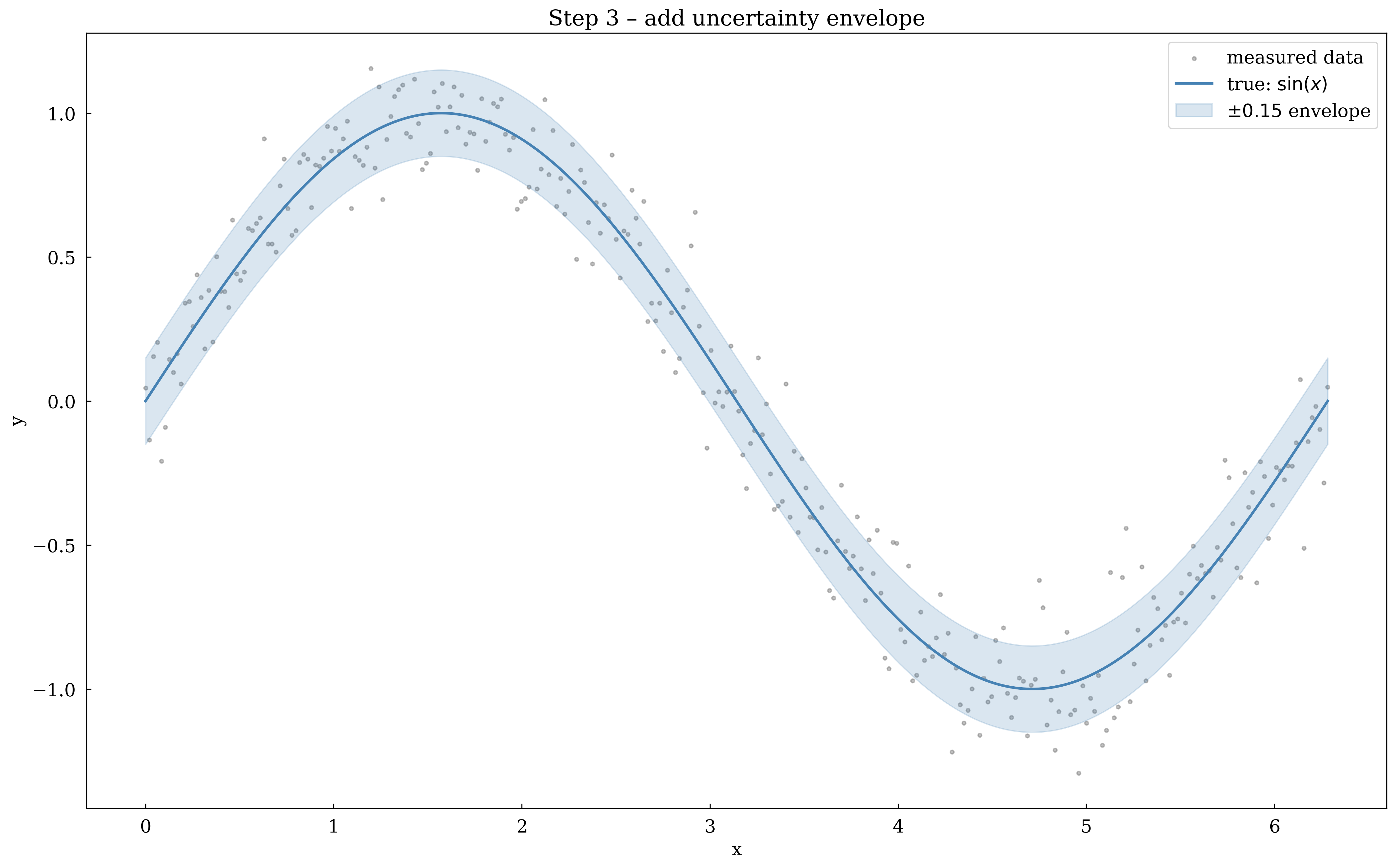
[10]:
# Step 3: add the uncertainty envelope
ax.set_title("Step 3 – add uncertainty envelope")
canvas.show(backend=BACKEND, layers=[0, 1, 2])

Summary
Concept |
How |
|---|---|
Assign to layer |
|
Render subset |
|
Save all layers |
|
Default layer |
|
Layers make it easy to build slide-deck animations or incremental pedagogical figures from a single Python file.