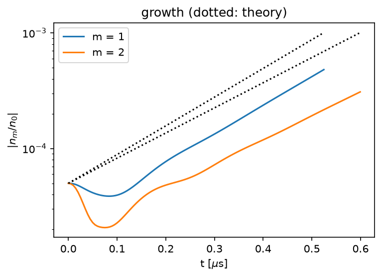
Verification of the 2D drift fluid: a uniform state, the E x B drift and a linear instability.

Three checks of :class:wellbalanced.DriftFluid2D against theory, each in seconds:

1. a state uniform along y stays uniform to round-off (the symmetry of the scheme);
2. a passive density blob in a uniform E and B drifts at E/B along y;
3. in a uniform plasma periodic in x and y an azimuthal perturbation grows with the growth rate and the frequency of the full-Poisson local dispersion relation (:func:wellbalanced.driftfluid2d.uniform_plasma_roots).

The Boeuf-case science (spokes, seeds, scans) is in the magnetron gallery, not here.

Python source

"""Verification of the 2D drift fluid: a uniform state, the E x B drift and a linear instability.

Three checks of :class:`wellbalanced.DriftFluid2D` against theory, each in seconds:

1. a state uniform along ``y`` stays uniform to round-off (the symmetry of the scheme);
2. a passive density blob in a uniform ``E`` and ``B`` drifts at ``E/B`` along ``y``;
3. in a uniform plasma periodic in ``x`` and ``y`` an azimuthal perturbation grows with the
   growth rate and the frequency of the full-Poisson local dispersion relation
   (:func:`wellbalanced.driftfluid2d.uniform_plasma_roots`).

The Boeuf-case science (spokes, seeds, scans) is in the magnetron gallery, not here.
"""

import matplotlib.pyplot as plt
import numpy as np

from wellbalanced import DriftFluid2D
from wellbalanced.driftfluid2d import (
    exponential_field,
    fit_mode,
    uniform_plasma_roots,
)

E = 1.602176634e-19

# 1. a y-uniform state stays uniform
model = DriftFluid2D(
    0.02,
    0.016,
    16,
    8,
    voltage=260.0,
    magnetic_field=exponential_field(0.12, 0.006),
    electron_temperature=None,
)
profile = 1e15 * np.exp(-(((model.x - 0.012) / 0.004) ** 2)) + 1e13
state = model.initial_state(profile[:, None] * np.ones((1, model.ny)))
step = model.suggest_timestep(state)
for _ in range(15):
    state = model.step(state, step)
spread = np.abs(
    state.electron_density - state.electron_density.mean(axis=1, keepdims=True)
).max()
print(
    f"1. variation along y after 15 steps: {spread / state.electron_density.max():.1e}"
)

# 2. the E x B drift of a passive blob
tracer = DriftFluid2D(
    0.02,
    0.04,
    20,
    64,
    voltage=100.0,
    magnetic_field=0.05,
    momentum_rate=1e-20,
    electron_temperature=1e-3,
)
x, y = np.meshgrid(tracer.x, tracer.y, indexing="ij")
floor = 1e10
density = 1e15 * np.exp(-((x - 0.01) ** 2 + (y - 0.02) ** 2) / 0.004**2) + floor
tracer_state = tracer.initial_state(density)
fields = tracer._fields(tracer_state.potential)
v_exb = -fields[4].mean() / 0.05


def rhs(n):
    """The density tendency from the electron flux in the fixed field."""
    gx, gy, _ = tracer._electron_like_flux(
        n, tracer_state.electron_temperature, fields, tracer_state.gas_density
    )
    gx[0] = gx[-1] = 0.0
    return -(tracer._divx @ gx.ravel() + tracer._divy @ gy.ravel()).reshape(n.shape)


duration = 4e-8
steps = int(duration / (0.3 * tracer.dy / v_exb)) + 1
dt = duration / steps
n = density
for _ in range(steps):
    k1 = n + dt * rhs(n)
    k2 = 0.75 * n + 0.25 * (k1 + dt * rhs(k1))
    n = n / 3.0 + 2.0 / 3.0 * (k2 + dt * rhs(k2))
phase = np.angle(((n - floor).sum(axis=0) * np.exp(2j * np.pi * tracer.y / 0.04)).sum())
shift = (phase / (2 * np.pi) * 0.04 - 0.02 + 0.02) % 0.04 - 0.02
print(f"2. blob speed {shift / duration:.0f} m/s, E/B = {v_exb:.0f} m/s")

# 3. linear growth in a uniform plasma against the dispersion relation
density0, e_field, b_field = 1e16, -2200.0, 0.02
plasma = DriftFluid2D(
    0.0048,
    0.016,
    4,
    32,
    voltage=0.0,
    magnetic_field=b_field,
    gas_density=1.43e20,
    electron_temperature=5.0,
    momentum_rate=2e7 / 1.43e20,
    ion_friction_rate=1e6 / 1.43e20,
    ionization_rate=lambda te: 0.0 * te,
    refill_rate=0.0,
    secondary_emission=0.0,
    ion_temperature=1e-4,
    field_bc=e_field,
    periodic_x=True,
)
fig, ax = plt.subplots(figsize=(5, 3.6), constrained_layout=True)
for mode in (1, 2):
    start = plasma.initial_state(density0, electron_temperature=5.0)
    start.ion_velocity[0] = E * e_field / (plasma.ion_mass * 1e6)
    start = plasma.step(start, 1e-13)
    plasma.stationary_sources(start)
    k = 2 * np.pi * mode / plasma.length_y
    wave = 1.0 + 1e-4 * np.cos(k * plasma.y)[None, :]
    start.electron_density = start.electron_density * wave
    start.ion_density = start.ion_density * wave
    roots = uniform_plasma_roots(
        0.0, k, density0, e_field, b_field, 5.0, plasma.ion_mass, 1e6, 2e7
    )
    growing = roots[np.argmax(roots.real)]
    t_end = 3.0 / growing.real
    run = plasma.run(start, t_end, record_every=t_end / 120)
    fit = fit_mode(
        run.times, run.amplitudes, mode, plasma.length_y, (0.45 * t_end, t_end)
    )
    print(
        f"3. m = {mode}: growth {fit.growth_rate:.3e} /s (theory {growing.real:.3e}), "
        f"frequency {fit.frequency:.3e} rad/s (theory {-growing.imag:.3e})"
    )
    ax.semilogy(run.times * 1e6, np.abs(run.amplitudes[:, mode]), label=f"m = {mode}")
    ax.semilogy(
        run.times * 1e6,
        np.abs(run.amplitudes[0, mode]) * np.exp(growing.real * run.times),
        "k:",
    )
ax.set_xlabel("t [$\\mu$s]")
ax.set_ylabel("$|n_m / n_0|$")
ax.set_title("growth (dotted: theory)")
ax.legend()

Plots