A global model of a HiPIMS magnetron: rarefaction, metal ions and self-sputtering.

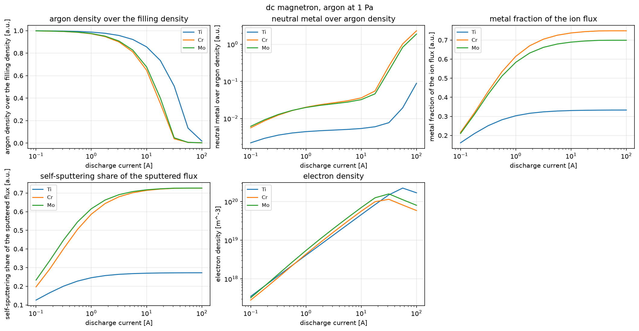
The ionization region of a sputtering magnetron in argon, balanced as a global model: Ar and the sputtered metal, ionized by the electrons the secondary electrons heat, lost at the Bohm speed through the target (where the ions sputter it, by Ar+ and, for self-sputtering, by the metal ions) and through the sides, with the argon replaced on a refill time and pushed out by the sputtered atoms (the sputter wind). Driven by the discharge current and voltage of an experiment, it returns what decides the spoke regime: the argon rarefaction, the metal to argon density ratio, the metal share of the ion flux, the self-sputtering share of the sputtered flux and the electron density. 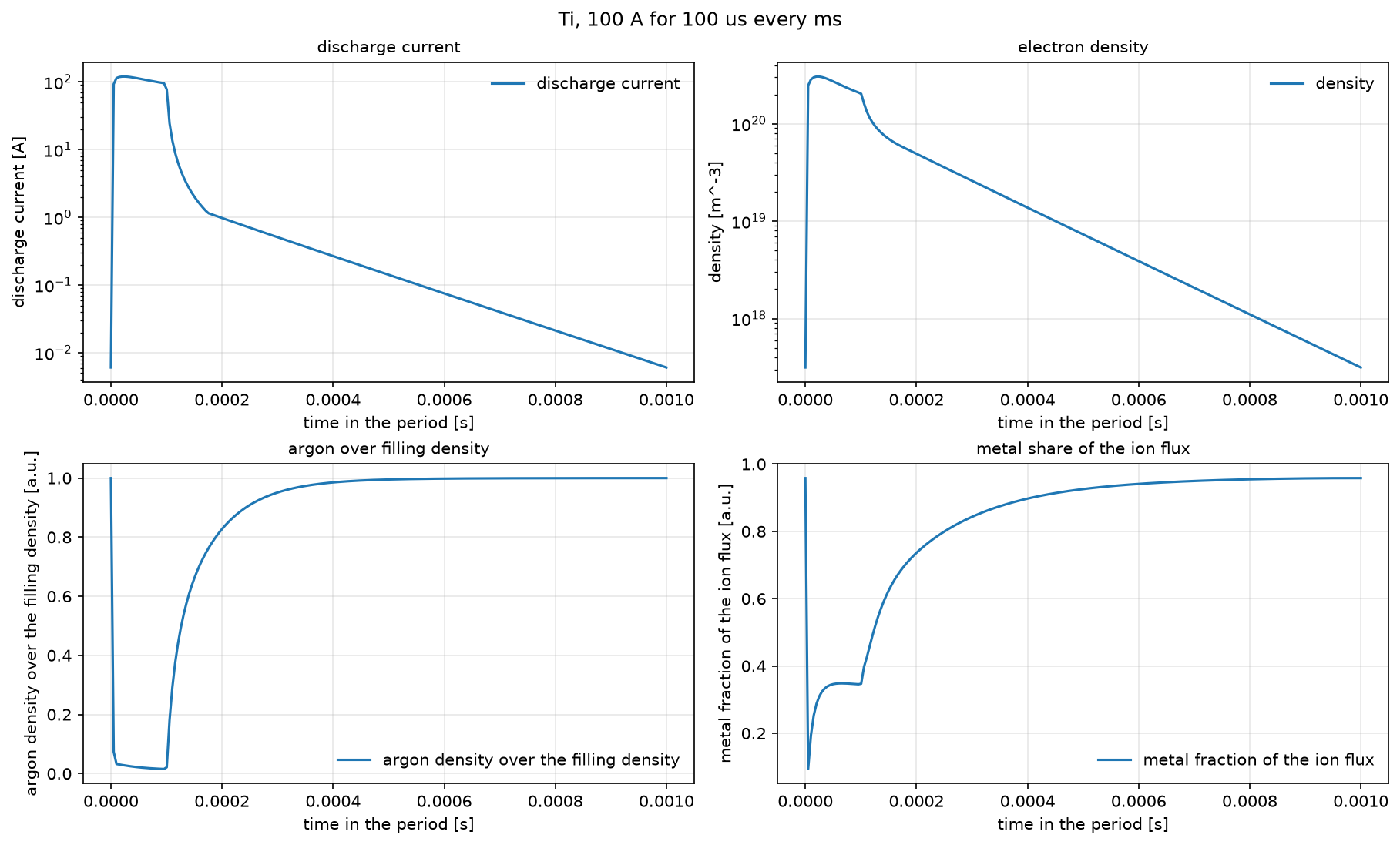First the dc states from 0.1 to 100 A for three targets, then a 100 A, 100 us pulse every millisecond on titanium, brought to its periodic state. The sputter and secondary electron yields, the geometry, the sputter wind and the heating are placeholders (see wellbalanced.magnetron): the trends are the model’s, the numbers are not data.

Python source

"""A global model of a HiPIMS magnetron: rarefaction, metal ions and self-sputtering.

The ionization region of a sputtering magnetron in argon, balanced as a global model: Ar
and the sputtered metal, ionized by the electrons the secondary electrons heat, lost at the
Bohm speed through the target (where the ions sputter it, by ``Ar+`` and, for
self-sputtering, by the metal ions) and through the sides, with the argon replaced on a
refill time and pushed out by the sputtered atoms (the sputter wind). Driven by the
discharge current and voltage of an experiment, it returns what decides the spoke regime:
the argon rarefaction, the metal to argon density ratio, the metal share of the ion flux,
the self-sputtering share of the sputtered flux and the electron density. First the dc
states from 0.1 to 100 A for three targets, then a 100 A, 100 us pulse every millisecond
on titanium, brought to its periodic state. The sputter and secondary electron yields,
the geometry, the sputter wind and the heating are placeholders (see
``wellbalanced.magnetron``): the trends are the model's, the numbers are not data.
"""

import warnings

import numpy as np
import plasma_plots
import xarray as xr

from wellbalanced.magnetron import MATERIALS, Magnetron

warnings.filterwarnings("ignore", message=".*placeholders, not data")


def voltage(current: float) -> float:
    """A placeholder current-voltage characteristic, 400 V at 0.1 A rising slowly."""
    return 400.0 + 60.0 * np.log10(1.0 + current)


currents = np.geomspace(0.1, 100.0, 13)
scans = []
for name in ("Ti", "Cr", "Mo"):
    magnetron = Magnetron(material=MATERIALS[name], wind_efficiency=0.3)
    # the heating fraction is fitted to a 2 A point, the others are predictions
    magnetron = magnetron.calibrate_heating(2.0, voltage(2.0))
    scans.append(magnetron.current_scan(currents, voltage))
dc = xr.concat(scans, dim="material", join="outer").assign_coords(
    material=["Ti", "Cr", "Mo"]
)

diagnostics = (
    ("rarefaction", False),
    ("metal_to_argon", True),
    ("metal_ion_fraction", False),
    ("self_sputtering_share", False),
    ("electron_density", True),
)
with plasma_plots.figure(2, 3, title="dc magnetron, argon at 1 Pa") as fig:
    for k, (name, logy) in enumerate(diagnostics):
        dc[name].plasma.plot.profiles(
            x="current", over="material", logx=True, logy=logy, ax=fig[k]
        )

titanium = Magnetron(wind_efficiency=0.3).calibrate_heating(2.0, voltage(2.0))
pulse = titanium.pulse(
    current=100.0, voltage=700.0, on_time=100.0e-6, period=1.0e-3, periods=20
)
end = pulse.sel(t=pulse.attrs["on_time"], method="nearest")
print(
    f"periodic after {pulse.attrs['periods']} pulses "
    f"(change {pulse.attrs['periodicity_error']:.1e}); at the end of the pulse: "
    f"I_D = {float(end.I_D):.0f} A, argon at {float(end.rarefaction):.2f} of the "
    f"filling density, metal ion flux fraction {float(end.metal_ion_fraction):.2f}"
)
with plasma_plots.figure(2, 2, title="Ti, 100 A for 100 us every ms") as fig:
    pulse.I_D.plasma.plot.timeseries(logy=True, title="discharge current", ax=fig[0])
    pulse.density.sel(species="e").plasma.plot.timeseries(
        logy=True, title="electron density", ax=fig[1]
    )
    pulse.rarefaction.plasma.plot.timeseries(
        logy=False, title="argon over filling density", ax=fig[2]
    )
    pulse.metal_ion_fraction.plasma.plot.timeseries(
        logy=False, title="metal share of the ion flux", ax=fig[3]
    )

Plots