The RF field of one and two drivers with a prescribed plasma: mutual coupling and shields.

The geometry of Zielke, Briefi and Fantz (NIBS’22, arXiv:2211.10143, Fig. 2): a horizontal 2D cut through a driver (23.7 cm wide, 17.4 cm long) and the expansion region (24.4 cm), six coil windings (6 mm tubes) on each side, 1 MHz; the backplates and the expansion walls are perfect conductors, and so are the electromagnetic shields (EMS) when present. With :class:wellbalanced.spatial.InductiveField2D and a prescribed plasma shaped like their Fig. 3 (up to 1.4e18 m^-3, depleted at the coil), this computes:

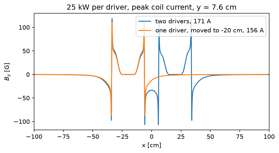
1. |B_y| along the line through the coil centres, one driver and two (their Fig. 4): the second driver raises the field at the coils;
2. the coil current for 25 kW absorbed per driver and the RF power transfer efficiency, one driver and two (their 263 A and 284 A, 55 % and 50 %);
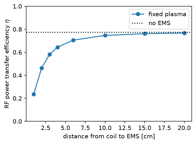
3. the efficiency against the distance between the coil and the shield (their Fig. 6).

With the plasma held fixed, only the mechanism and the trends are expected, not the numbers: the paper’s plasma follows the field (the RF Lorentz force pushes it from the coil), and its 2D-to-3D conversion is not stated. Here the power of a driver is the power per unit length of the cut times DEPTH = pi times the driver radius (the half circumference, where the skin layer is), and the collision frequency is a placeholder of the right order (1e7 /s, from an e-H2 momentum-transfer cross section of about 1e-19 m^2 at 10 eV on 4.5e19 m^-3 of gas).

Python source

"""The RF field of one and two drivers with a prescribed plasma: mutual coupling and shields.

The geometry of Zielke, Briefi and Fantz (NIBS'22, arXiv:2211.10143, Fig. 2): a
horizontal 2D cut through a driver (23.7 cm wide, 17.4 cm long) and the expansion region
(24.4 cm), six coil windings (6 mm tubes) on each side, 1 MHz; the backplates and the
expansion walls are perfect conductors, and so are the electromagnetic shields (EMS) when
present. With :class:`wellbalanced.spatial.InductiveField2D` and a *prescribed* plasma
shaped like their Fig. 3 (up to 1.4e18 m^-3, depleted at the coil), this computes:

1. ``|B_y|`` along the line through the coil centres, one driver and two (their Fig. 4):
   the second driver raises the field at the coils;
2. the coil current for 25 kW absorbed per driver and the RF power transfer efficiency,
   one driver and two (their 263 A and 284 A, 55 % and 50 %);
3. the efficiency against the distance between the coil and the shield (their Fig. 6).

With the plasma held fixed, only the mechanism and the trends are expected, not the
numbers: the paper's plasma follows the field (the RF Lorentz force pushes it from the
coil), and its 2D-to-3D conversion is not stated. Here the power of a driver is the power
per unit length of the cut times ``DEPTH`` = pi times the driver radius (the half
circumference, where the skin layer is), and the collision frequency is a placeholder of
the right order (1e7 /s, from an e-H2 momentum-transfer cross section of about 1e-19 m^2
at 10 eV on 4.5e19 m^-3 of gas).
"""

import matplotlib.pyplot as plt
import numpy as np
from simgeometry import Circle, Rectangle

from wellbalanced.spatial import (
    Conductor,
    InductiveField2D,
    Winding,
    stretched_edges,
)

FREQUENCY = 1.0e6
HALF_WIDTH = 0.237 / 2  # driver plasma
DRIVER_LENGTH = 0.174
EXPANSION = 0.244
COIL_OFFSET = 0.1395  # winding centre from the driver axis: 2.1 cm outside the plasma
TUBE_RADIUS = 0.003
WINDING_PITCH = 0.022
WALL = 0.01  # backplate and wall thickness
SHIELD = 0.002  # EMS thickness
N_PEAK = 1.4e18
COLLISION_FREQUENCY = 1.0e7  # placeholder
DEPTH = np.pi * HALF_WIDTH
NETWORK_RESISTANCE = 0.6  # per driver, measured at BUG
POWER = 25e3  # absorbed per driver
SPACING = 1.0e-3


def box(x0, x1, y0, y1):
    """A rectangle from its bounds."""
    return Rectangle(((x0 + x1) / 2, (y0 + y1) / 2), (x1 - x0, y1 - y0))


def source(centres, expansion_half, shield_distance=None):
    """The windings, conductors and plasma of drivers at ``centres``."""
    windings, conductors = [], []
    plate_top = DRIVER_LENGTH - WALL
    for k, xc in enumerate(centres):
        for side, sign in ((-1.0, 1.0), (1.0, -1.0)):
            for n in range(6):
                y = DRIVER_LENGTH / 2 + (n - 2.5) * WINDING_PITCH
                windings.append(
                    Winding(Circle((xc + side * COIL_OFFSET, y), TUBE_RADIUS), sign)
                )
        outer = HALF_WIDTH + 0.006  # the dielectric driver wall
        conductors.append(
            Conductor(
                [box(xc - outer, xc + outer, -WALL, 0.0)], name=f"driver backplate {k}"
            )
        )
        if shield_distance is not None:
            plates = [
                box(x - SHIELD / 2, x + SHIELD / 2, -WALL, plate_top)
                for x in (
                    xc - COIL_OFFSET - shield_distance,
                    xc + COIL_OFFSET + shield_distance,
                )
            ]
            conductors.append(Conductor(plates, name=f"shield {k}"))
    # the source backplate around the driver openings, the expansion walls and grid
    openings = sorted(
        (xc - HALF_WIDTH - 0.006, xc + HALF_WIDTH + 0.006) for xc in centres
    )
    edges = [-expansion_half, *[x for pair in openings for x in pair], expansion_half]
    pieces = [
        box(edges[i], edges[i + 1], plate_top, DRIVER_LENGTH)
        for i in range(0, len(edges), 2)
        if edges[i + 1] > edges[i]
    ]
    top = DRIVER_LENGTH + EXPANSION
    pieces += [
        box(-expansion_half - WALL, -expansion_half, plate_top, top + WALL),
        box(expansion_half, expansion_half + WALL, plate_top, top + WALL),
        box(-expansion_half, expansion_half, top, top + WALL),
    ]
    conductors.append(Conductor(pieces, name="source"))

    def density(x, y):
        n = np.zeros_like(x)
        for xc in centres:
            inside = (np.abs(x - xc) < HALF_WIDTH) & (y > 0.0) & (y < DRIVER_LENGTH)
            radial = np.cos(0.5 * np.pi * (x - xc) / HALF_WIDTH) ** 2
            axial = 0.35 + 0.65 * np.sin(0.5 * np.pi * np.minimum(y / 0.15, 1.0))
            n = np.where(inside, N_PEAK * radial * axial, n)
        lobes = sum(
            np.cos(0.5 * np.pi * (x - xc) / (HALF_WIDTH + 0.05)) ** 2
            * (np.abs(x - xc) < HALF_WIDTH + 0.05)
            for xc in centres
        )
        expansion = (np.abs(x) < expansion_half) & (y >= DRIVER_LENGTH) & (y < top)
        decay = np.exp(-(y - DRIVER_LENGTH) / 0.12)
        return np.where(expansion, N_PEAK * (0.15 + 0.6 * lobes * decay), n)

    return windings, conductors, density


def model(centres, expansion_half, shield_distance=None, fine_half=0.36):
    """The field model, 1 mm cells over the source, stretched to a 2.4 m box."""
    windings, conductors, density = source(centres, expansion_half, shield_distance)
    x_edges = stretched_edges(-1.2, 1.2, -fine_half, fine_half, SPACING, ratio=1.06)
    y_edges = stretched_edges(-0.8, 1.2, -0.03, 0.44, SPACING, ratio=1.06)
    return InductiveField2D(
        x_edges,
        y_edges,
        frequency=FREQUENCY,
        windings=windings,
        conductors=conductors,
        electron_density=density,
        collision_frequency=COLLISION_FREQUENCY,
    )


def at_power(field_model, drivers):
    """The solution with ``POWER`` absorbed per driver, its efficiency and |B_y|."""
    solution = field_model.solve(1.0).for_power(drivers * POWER, DEPTH)
    eta = solution.efficiency(drivers * NETWORK_RESISTANCE, DEPTH)
    return solution, eta


single = model([0.0], 0.16)
double = model([-0.20, 0.20], 0.43, fine_half=0.47)
one, eta_one = at_power(single, 1)
two, eta_two = at_power(double, 2)
print("                    this model (fixed plasma)   Zielke et al. (self-consistent)")
print(f"coil current, 1 driver   {abs(one.coil_current):6.0f} A               263 A")
print(f"coil current, 2 drivers  {abs(two.coil_current):6.0f} A               284 A")
print(f"efficiency,   1 driver   {eta_one:6.1%}                 55 %")
print(f"efficiency,   2 drivers  {eta_two:6.1%}                 50 %")
print(
    f"plasma resistance per driver: {one.plasma_resistance(DEPTH):.3f} Ohm (1), "
    f"{two.plasma_resistance(DEPTH) / 2:.3f} Ohm (2)"
)

# 1. B_y along a row of winding centres at peak coil current (Fig. 4)
y_row = DRIVER_LENGTH / 2 - 0.5 * WINDING_PITCH  # the third winding from the bottom


def field_on_row(solution, shift=0.0):
    """The x coordinates and the instant B_y at peak coil current on the winding row."""
    j = np.argmin(np.abs(solution.y - y_row))
    _, b_y = solution.magnetic_field
    return (solution.x + shift), np.real(b_y[:, j])  # the instant of peak current


fig, ax = plt.subplots(figsize=(7, 3.5))
for solution, label, shift in (
    (two, "two drivers", 0.0),
    (one, "one driver, moved to -20 cm", -0.20),
):
    x, b = field_on_row(solution, shift)
    ax.plot(x * 100, b * 1e4, label=f"{label}, {abs(solution.coil_current):.0f} A")
ax.set_xlim(-100, 100)
ax.set_xlabel("x [cm]")
ax.set_ylabel("$B_y$ [G]")
ax.set_title(f"25 kW per driver, peak coil current, y = {y_row * 100:.1f} cm")
ax.legend()
# the coupling at the same coil current: the field just inside the gap between the
# drivers, beside the left driver's inner coil (x = -6 cm), against the single driver
inner_coil = -0.20 + COIL_OFFSET
for solution, name, shift in (
    (one.scaled(1.0), "one driver", -0.20),
    (two.scaled(1.0), "two drivers", 0.0),
):
    x, b = field_on_row(solution, shift)
    beside = (x > inner_coil + TUBE_RADIUS) & (x < inner_coil + 3 * TUBE_RADIUS)
    print(
        f"B_y beside the inner coil per A of coil current, {name}: "
        f"{np.abs(b[beside]).max() * 1e4:.3f} G/A"
    )

# 2. the efficiency against the coil-shield distance (Fig. 6), one driver
distances = np.array([0.01, 0.02, 0.03, 0.04, 0.06, 0.10, 0.15, 0.20])
efficiencies = []
for distance in distances:
    shielded = model([0.0], 0.16, shield_distance=distance)
    efficiencies.append(at_power(shielded, 1)[1])
print("coil-EMS distance [cm]: " + " ".join(f"{d * 100:5.0f}" for d in distances))
print("efficiency, this model: " + " ".join(f"{e:5.2f}" for e in efficiencies))
print(
    "Zielke et al. Fig. 6:      0.21  0.31  0.41  0.46  0.50  0.54  0.54  0.54 (read off)"
)
print(f"no EMS: {eta_one:.2f} (Zielke: 0.55)")
fig, ax = plt.subplots(figsize=(5, 3.5))
ax.plot(distances * 100, efficiencies, "o-", label="fixed plasma")
ax.axhline(eta_one, color="k", ls=":", label="no EMS")
ax.set_xlabel("distance from coil to EMS [cm]")
ax.set_ylabel(r"RF power transfer efficiency $\eta$")
ax.set_ylim(0, 1)
ax.legend()

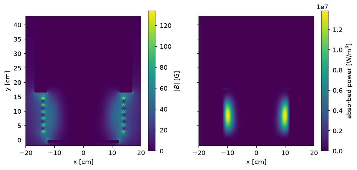
# the field and the absorbed power of one driver
fig, axes = plt.subplots(1, 2, figsize=(9, 4), sharey=True)
b_x, b_y = one.magnetic_field
window = (np.abs(one.x) < 0.2)[:, None] & ((one.y > -0.02) & (one.y < 0.43))[None, :]
xs, ys = one.x[np.abs(one.x) < 0.2], one.y[(one.y > -0.02) & (one.y < 0.43)]
shape = (xs.size, ys.size)
for ax, values, title in (
    (axes[0], np.hypot(np.abs(b_x), np.abs(b_y)), "$|B|$ [G]"),
    (axes[1], one.power_density, "absorbed power [W/m$^3$]"),
):
    data = values[window].reshape(shape).T
    image = ax.pcolormesh(xs * 100, ys * 100, data * (1e4 if "G" in title else 1.0))
    fig.colorbar(image, ax=ax, label=title)
    ax.set_xlabel("x [cm]")
    ax.set_aspect("equal")
axes[0].set_ylabel("y [cm]")

Plots