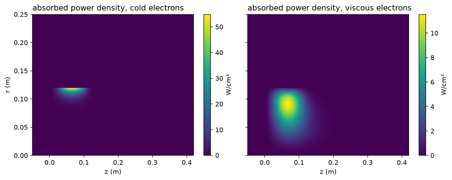
The BUG driver in r–z: cold and viscous electrons, and the global model's plasma.
The 2D cylindrically symmetric domain of Zielke, Briefi, Lishev and Fantz (Plasma Sources
Sci. Technol. 31, 035019, 2022, Fig. 1(b), dimensions read off the figure): the driver
(radius 12 cm, 17 cm long) opening into the expansion region (radius 19 cm, up to the
plasma grid at 42 cm), the driver and source backplates and the expansion wall as
perfect conductors, the plasma grid as the right edge of the domain, the surroundings up
to r = 50 cm; six coil turns (6 mm tubes) around the driver, 1 MHz,
R_net = 0.6 Ohm. With :class:wellbalanced.spatial.InductiveField2D in r–z (no
2D-to-3D depth) this computes:
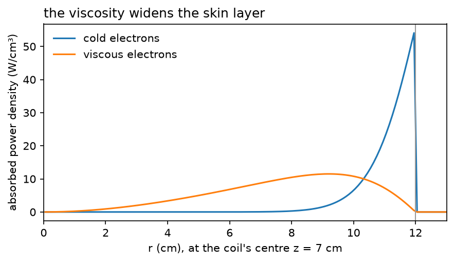
- the coil current and the RF power transfer efficiency at 25 kW absorbed, for a prescribed plasma (peak 1e18 m^-3, 10 eV) with (a) cold electrons and (b) the collisional viscosity of the paper’s eq. 7, against steps R1 (x–y cut) and R2 (0D);
- (c) the global model of :func:
wellbalanced.driver.illustrative_hydrogen_driverin this field (:func:wellbalanced.spatial.global_model_plasmaon the same shape) at the paper’s operating point, 60 kW from the generator at 0.3 Pa, where they reportI_RF ≈ 250 Aandeta ≈ 60 %(model and measurement).
Everything runs on two grids: a tensor grid of 1 mm cells over the source, stretched
toward the far boundary, and refined patches (:class:wellbalanced.spatial.PatchGrid, on
patchwork): a 4 mm base out to the far boundary, 2 mm over the source and its
conductors, 1 mm over the coil and the driver’s skin layer. The patches give the same
numbers with about a third of the cells; one more level where the cold plasma absorbs
(:meth:~wellbalanced.spatial.PatchGrid.refined_where) shows the skin layer resolved.
Still missing for the paper’s model: the RF Lorentz force, which pushes the plasma off
the coil (it needs the in-plane electron flux of Fluid2D), the plasma and neutral
fluids themselves (here the plasma’s shape is prescribed), and real hydrogen rates (the
global model’s are placeholders). The electrons’ no-slip edge is an assumption, and the
geometry is read off a figure.
Python source
Section titled “Python source”"""The BUG driver in r–z: cold and viscous electrons, and the global model's plasma.
The 2D cylindrically symmetric domain of Zielke, Briefi, Lishev and Fantz (Plasma SourcesSci. Technol. 31, 035019, 2022, Fig. 1(b), dimensions read off the figure): the driver(radius 12 cm, 17 cm long) opening into the expansion region (radius 19 cm, up to theplasma grid at 42 cm), the driver and source backplates and the expansion wall asperfect conductors, the plasma grid as the right edge of the domain, the surroundings upto r = 50 cm; six coil turns (6 mm tubes) around the driver, 1 MHz,``R_net = 0.6`` Ohm. With :class:`wellbalanced.spatial.InductiveField2D` in r–z (no2D-to-3D depth) this computes:
1. the coil current and the RF power transfer efficiency at 25 kW absorbed, for a prescribed plasma (peak 1e18 m^-3, 10 eV) with (a) cold electrons and (b) the collisional viscosity of the paper's eq. 7, against steps R1 (x–y cut) and R2 (0D);2. (c) the global model of :func:`wellbalanced.driver.illustrative_hydrogen_driver` in this field (:func:`wellbalanced.spatial.global_model_plasma` on the same shape) at the paper's operating point, 60 kW from the generator at 0.3 Pa, where they report ``I_RF ≈ 250 A`` and ``eta ≈ 60 %`` (model and measurement).
Everything runs on two grids: a tensor grid of 1 mm cells over the source, stretchedtoward the far boundary, and refined patches (:class:`wellbalanced.spatial.PatchGrid`, onpatchwork): a 4 mm base out to the far boundary, 2 mm over the source and itsconductors, 1 mm over the coil and the driver's skin layer. The patches give the samenumbers with about a third of the cells; one more level where the cold plasma absorbs(:meth:`~wellbalanced.spatial.PatchGrid.refined_where`) shows the skin layer resolved.
Still missing for the paper's model: the RF Lorentz force, which pushes the plasma offthe coil (it needs the in-plane electron flux of ``Fluid2D``), the plasma and neutralfluids themselves (here the plasma's shape is prescribed), and real hydrogen rates (theglobal model's are placeholders). The electrons' no-slip edge is an assumption, and thegeometry is read off a figure."""
import timeimport warnings
import matplotlib.pyplot as pltimport numpy as npfrom simgeometry import Circle, Rectangle
from wellbalanced.driver import illustrative_hydrogen_driverfrom wellbalanced.spatial import ( Conductor, DriverCoupling, InductiveField2D, PatchGrid, PlasmaProfile, PlasmaRegion, Winding, global_model_plasma, stretched_edges,)
FREQUENCY = 1.0e6DRIVER_RADIUS, DRIVER_END = 0.12, 0.17EXPANSION_RADIUS, GRID = 0.19, 0.42COIL_RADIUS, TUBE_RADIUS = 0.128, 0.003COIL_Z = np.linspace(0.035, 0.10, 6)NETWORK_RESISTANCE = 0.6SPACING = 1.0e-3
def box(r0, r1, z0, z1): """A rectangle from its bounds.""" return Rectangle(((r0 + r1) / 2, (z0 + z1) / 2), (r1 - r0, z1 - z0))
REGION = PlasmaRegion( [ box(0.0, DRIVER_RADIUS, 0.0, DRIVER_END), box(0.0, EXPANSION_RADIUS, DRIVER_END, GRID), ])WINDINGS = [ Winding(Circle((COIL_RADIUS, z), TUBE_RADIUS), name=f"turn {k}") for k, z in enumerate(COIL_Z)]CONDUCTORS = [ Conductor([box(0.0, 0.125, -0.04, 0.0)], name="driver backplate"), Conductor([box(0.125, 0.195, 0.125, DRIVER_END)], name="source backplate"), Conductor([box(0.19, 0.195, DRIVER_END, GRID)], name="expansion wall"),]
def shape(r, z): """The plasma's shape: peaked on the axis, a fifth of that at the driver wall.
It decays into the expansion region; its mean over the driver is 1. """ radial = 0.2 + 0.8 * np.cos(0.5 * np.pi * np.clip(r / DRIVER_RADIUS, 0.0, 1.0)) axial = np.where(z < DRIVER_END, 1.0, np.exp(-(z - DRIVER_END) / 0.08)) driver = (r < DRIVER_RADIUS) & (z > 0.0) & (z < DRIVER_END) mean = 0.2 + 0.8 * (8.0 / np.pi**2) * (np.pi / 2 - 1.0) # of the radial part return np.where(driver | (z >= DRIVER_END), radial * axial / mean, 0.0)
# The two grids: the tensor grid's edges, or the patches (made once, for every field).GRIDS = { "stretched": { "x_edges": stretched_edges(0.0, 0.5, 0.0, 0.2, SPACING, ratio=1.08), "y_edges": stretched_edges(-0.135, GRID, -0.045, GRID, SPACING, ratio=1.08), "geometry": "cylindrical", }, "patches": { "grid": PatchGrid.refined( ((0.0, 0.5), (-0.14, GRID)), (125, 140), # 4 mm [ [((0.0, 0.2), (-0.045, GRID))], # 2 mm: the source and its conductors [((0.08, 0.14), (-0.01, 0.18))], # 1 mm: the coil, the skin layer ], geometry="cylindrical", ) },}
def field(profile: PlasmaProfile, grid: str = "stretched") -> InductiveField2D: """The r–z field of the BUG driver for a plasma, on one of the two grids.""" return InductiveField2D( **GRIDS[grid], frequency=FREQUENCY, windings=WINDINGS, conductors=CONDUCTORS, plasma_region=REGION, **profile.settings(), )
# --- 1. a prescribed plasma at 25 kW: cold and viscous electrons ---------------------N_PEAK, T_E, NU = 1.0e18, 10.0, 1.0e7 # the collision frequency is a placeholder
prescribed, prescribed_patches, cells, seconds = {}, {}, {}, {}for grid, results in (("stretched", prescribed), ("patches", prescribed_patches)): start = time.perf_counter() for name, temperature in (("cold", None), ("viscous", T_E)): profile = PlasmaProfile( lambda r, z: N_PEAK * shape(r, z) / shape(0.0, 0.05), NU, temperature ) model = field(profile, grid) results[name] = model.solve(1.0).for_power(25e3) cells[grid] = model.grid.size seconds[grid] = time.perf_counter() - start
print("25 kW absorbed coil current eta viscous share (patches)")for name, solution in prescribed.items(): share = solution.viscous_power / solution.absorbed_power patches = prescribed_patches[name] print( f"r–z, {name:8s} {abs(solution.coil_current):6.0f} A " f"{solution.efficiency(NETWORK_RESISTANCE):5.1%} {share:6.1%} " f"{abs(patches.coil_current):6.0f} A " f"{patches.efficiency(NETWORK_RESISTANCE):5.1%}" )print("R1, x–y cut, cold 156 A 77.4 % (assumed depth)")print("R2, 0D transformer 203 A 67.0 %")print("Zielke et al., NIBS'22 263 A 55 % (x–y, self-consistent)")
# --- 2. the global model's plasma at 60 kW from the generator -----------------------with warnings.catch_warnings(): warnings.simplefilter("ignore", UserWarning) # placeholder rates, said above driver = illustrative_hydrogen_driver()coupled: dict[str, dict] = {"stretched": {}, "patches": {}}for grid in coupled: start = time.perf_counter() for name, viscous in (("cold", False), ("viscous", True)): model = DriverCoupling( field=lambda profile, grid=grid: field(profile, grid), plasma=global_model_plasma(driver, shape, viscous=viscous), network_resistance=NETWORK_RESISTANCE, ) coupled[grid][name] = model.at_rf_power(60e3, tolerance=1e-4, relaxation=0.7) seconds[grid] += time.perf_counter() - start
print( "\n60 kW generator absorbed coil current eta n_e (driver) T_e passes")for grid, states in coupled.items(): for name, state in states.items(): plasma = state.plasma.plasma print( f"{grid:9s} {name:8s} {state.absorbed_power / 1e3:5.1f} kW " f"{state.coil_current:6.0f} A {state.efficiency:5.1%} " f"{plasma.electron_density:9.2e} {plasma.electron_temperature:4.1f} " f"{state.iterations}" )transformer = coupled["stretched"]["cold"].plasmaprint( f"transformer model, same plasma: {transformer.coil_current:.0f} A, " f"eta {transformer.efficiency:.1%}")print( "Zielke et al. 2022, BUG, 0.3 Pa: about 250 A, eta about 60 % (model and measurement)")print("\ngrid cells time (all of the above)")for grid in GRIDS: print(f"{grid:9s} {cells[grid]:7d} {seconds[grid]:5.1f} s")
# --- 3. one more level over the skin layer --------------------------------------------cold = PlasmaProfile(lambda r, z: N_PEAK * shape(r, z) / shape(0.0, 0.05), NU)patches = GRIDS["patches"]["grid"]skin = prescribed_patches["cold"]finer = patches.refined_where(skin.power_density > 0.05 * skin.power_density.max())refined = InductiveField2D( grid=finer, frequency=FREQUENCY, windings=WINDINGS, conductors=CONDUCTORS, plasma_region=REGION, **cold.settings(),).solve(1.0)refined = refined.for_power(25e3)print( f"\nskin layer one level finer ({finer.size} cells, 0.5 mm): " f"{abs(refined.coil_current):.1f} A, eta {refined.efficiency(NETWORK_RESISTANCE):.2%} " f"(was {abs(skin.coil_current):.1f} A, {skin.efficiency(NETWORK_RESISTANCE):.2%})")
# --- figures ----------------------------------------------------------------------fig, axes = plt.subplots(1, 2, figsize=(10, 4), sharey=True)for ax, (name, solution) in zip(axes, prescribed.items(), strict=True): density = solution.power_density.T / 1e6 mesh = ax.pcolormesh( solution.y, solution.x, density.T, shading="auto", cmap="viridis" ) ax.set_xlim(-0.05, GRID) ax.set_ylim(0.0, 0.25) ax.set_xlabel("z (m)") ax.set_title(f"absorbed power density, {name} electrons", loc="left") fig.colorbar(mesh, ax=ax, label="W/cm³")axes[0].set_ylabel("r (m)")fig.tight_layout()
fig, ax = plt.subplots(figsize=(6, 3.5))for name, solution in prescribed.items(): j = int(np.argmin(np.abs(solution.y - 0.07))) ax.plot( solution.x * 100, solution.power_density[:, j] / 1e6, label=f"{name} electrons" )ax.axvline(DRIVER_RADIUS * 100, color="0.6", linewidth=1)ax.set_xlim(0, 13)ax.set_xlabel("r (cm), at the coil's centre z = 7 cm")ax.set_ylabel("absorbed power density (W/cm³)")ax.set_title("the viscosity widens the skin layer", loc="left")ax.legend(frameon=False)fig.tight_layout()