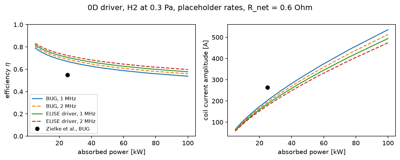
A 0D RF driver: coil current and RF power transfer efficiency in seconds.

:class:wellbalanced.RFDriver couples a global model of the driver’s hydrogen plasma to a transformer model of the coil (Piejak, Godyak and Alexandrovich 1992; Lieberman and Lichtenberg sec. 12.2): the absorbed power fixes the electron density and temperature, those fix the skin layer and the resistance the coil sees, and that the coil current and the efficiency eta = R_s / (R_s + R_net). Compared with Zielke, Briefi and Fantz (NIBS’22, arXiv:2211.10143) and with the 2D field of rf_driver_inductive_field_2d.py (step R1):

1. the BUG driver at 25 kW absorbed (their 263 A and 55 %);
2. 2 MHz instead of 1 MHz, and a 30 cm driver instead of 17 cm at the same coil (their Fig. 6 far from the shield: about 0.54, 0.67 and 0.82);
3. the coil current and efficiency against the absorbed power, BUG and ELISE drivers.

The rates are placeholders (illustrative_hydrogen_driver warns), the coil radius and the ion mean free path assumptions, and a 0D model has no shield and no second driver: the coil-shield distance and the mutual coupling of drivers (their Figs. 4-6) change the field around the coil, which is the 2D model’s part. Expect trends, not the paper’s numbers.

Python source

"""A 0D RF driver: coil current and RF power transfer efficiency in seconds.

:class:`wellbalanced.RFDriver` couples a global model of the driver's hydrogen plasma
to a transformer model of the coil (Piejak, Godyak and Alexandrovich 1992; Lieberman
and Lichtenberg sec. 12.2): the absorbed power fixes the electron density and
temperature, those fix the skin layer and the resistance the coil sees, and that the
coil current and the efficiency ``eta = R_s / (R_s + R_net)``. Compared with Zielke,
Briefi and Fantz (NIBS'22, arXiv:2211.10143) and with the 2D field of
``rf_driver_inductive_field_2d.py`` (step R1):

1. the BUG driver at 25 kW absorbed (their 263 A and 55 %);
2. 2 MHz instead of 1 MHz, and a 30 cm driver instead of 17 cm at the same coil (their
   Fig. 6 far from the shield: about 0.54, 0.67 and 0.82);
3. the coil current and efficiency against the absorbed power, BUG and ELISE drivers.

The rates are placeholders (``illustrative_hydrogen_driver`` warns), the coil radius
and the ion mean free path assumptions, and a 0D model has no shield and no second
driver: the coil-shield distance and the mutual coupling of drivers (their Figs. 4-6)
change the field around the coil, which is the 2D model's part. Expect trends, not
the paper's numbers.
"""

import dataclasses
import warnings

import matplotlib.pyplot as plt
import numpy as np

from wellbalanced.driver import illustrative_hydrogen_driver

with warnings.catch_warnings():
    warnings.simplefilter("ignore", UserWarning)  # the placeholder-data warning, once
    bug = illustrative_hydrogen_driver()
elise = dataclasses.replace(bug, radius=0.138, coil_radius=0.158)
POWER = 25.0e3

# 1. BUG at 25 kW
state = bug.solve(POWER)
exact = dataclasses.replace(bug, coupling="solenoid").couple(state.plasma, POWER)
plasma = state.plasma
print(
    f"BUG plasma at 25 kW: n_e = {plasma.electron_density:.2e} m^-3, "
    f"T_e = {plasma.electron_temperature:.2f} eV, nu_m = {state.collision_frequency:.2e} "
    f"/s, skin depth {state.skin_depth * 1e3:.1f} mm, coil factor {bug.coil.factor:.3f}"
)
print(
    "                      transformer   exact column   R1 2D (fixed plasma)   Zielke"
)
print(
    f"coil current [A]      {state.coil_current:8.0f}   {exact.coil_current:12.0f}"
    "                   156      263"
)
print(
    f"efficiency            {state.efficiency:8.1%}   {exact.efficiency:12.1%}"
    "                 77.4 %     55 %"
)
print(
    f"plasma resistance     {state.plasma_resistance:8.3f}   "
    f"{exact.plasma_resistance:12.3f} Ohm"
)
print(f"coil voltage [kV]     {state.coil_voltage / 1e3:8.1f}")

# 2. frequency and driver length (the coil stays 17 cm long)
print("\nefficiency at 25 kW      this model   Zielke Fig. 6, far from the shield")
cases = {
    "1 MHz, 17 cm": (bug, 0.54),
    "2 MHz, 17 cm": (dataclasses.replace(bug, frequency=2.0e6), 0.67),
    "1 MHz, 30 cm": (dataclasses.replace(bug, length=0.30, coil_length=0.17), 0.82),
}
for name, (driver, paper) in cases.items():
    print(f"{name}             {driver.solve(POWER).efficiency:8.3f}       {paper:.2f}")

# 3. against the absorbed power
powers = np.geomspace(5.0e3, 100.0e3, 12)
fig, (left, right) = plt.subplots(1, 2, figsize=(9, 3.6))
for name, driver in (("BUG", bug), ("ELISE driver", elise)):
    for frequency, style in ((1.0e6, "-"), (2.0e6, "--")):
        scan = dataclasses.replace(driver, frequency=frequency).scan("power", powers)
        label = f"{name}, {frequency / 1e6:.0f} MHz"
        left.plot(powers / 1e3, [s.efficiency for s in scan], style, label=label)
        right.plot(powers / 1e3, [s.coil_current for s in scan], style, label=label)
left.plot([25], [0.55], "ko", label="Zielke et al., BUG")
right.plot([25], [263], "ko")
left.set(xlabel="absorbed power [kW]", ylabel=r"efficiency $\eta$", ylim=(0, 1))
right.set(xlabel="absorbed power [kW]", ylabel="coil current amplitude [A]")
left.legend(fontsize=8)
fig.suptitle("0D driver, H2 at 0.3 Pa, placeholder rates, R_net = 0.6 Ohm")
fig.tight_layout()

Plots